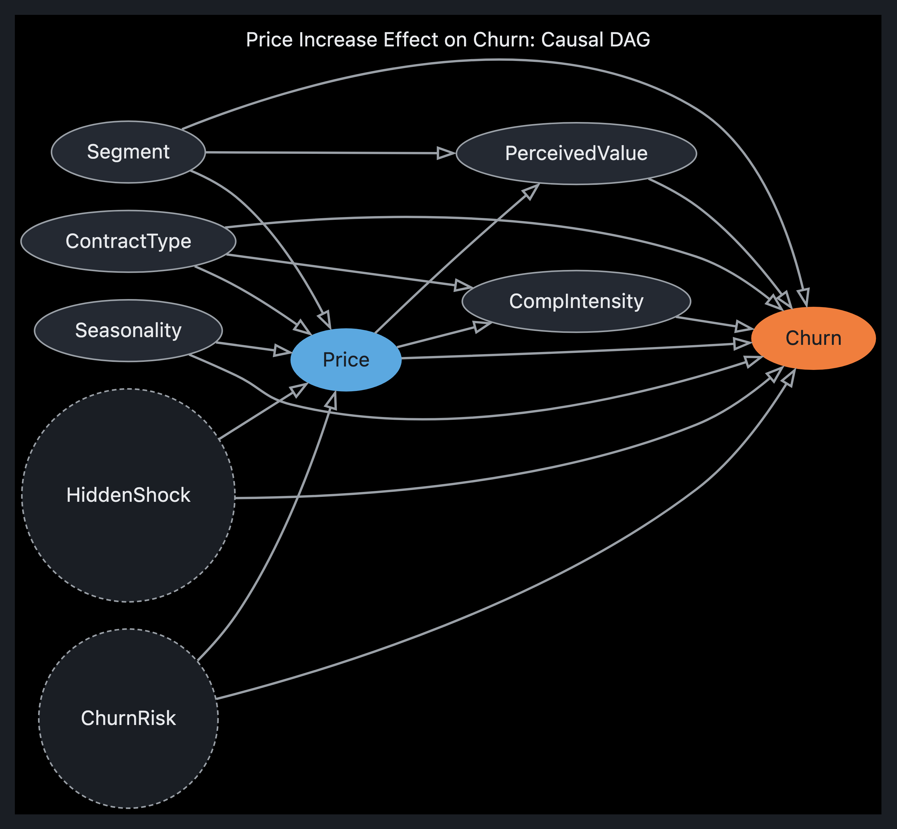
This is a clean backdoor-identification problem. Let me work it end to end: build the DAG, classify every node, enumerate the backdoor paths, run the do-calculus reduction, and give you a verdict on identifiability — with the assumption that actually decides it.
1. The DAG
Variables (with temporal ordering, which is what makes the structure defensible):
| Node | Role | Timing |
|---|
S Segment (enterprise / SMB / consumer) | confounder | pre-treatment, stable |
C Contract type (monthly / annual) | confounder (pre-treatment value) | pre-treatment |
T Seasonality (period of the price change) | confounder | pre-treatment |
P Price (the 15% increase) | treatment | — |
M Mediators (perceived value, usage drop, competitor-shopping, billing complaints) | mediator | post-treatment |
Y Churn | outcome | post-treatment |
U Unobserved (account-manager quality, customer financial health, latent price-sensitivity) | possible hidden confounder | pre-treatment |
Edges:
        S ───────────────┐
        │                 │
        ▼                 ▼
   ┌─── C ───────┐        │
   │    │        │        │
   ▼    ▼        ▼        ▼
   T ─► P ─────► M ─────► Y
        ▲                 ▲
        │                 │
        └──── U ──────────┘   (U dashed — unobserved)
Reading the edges:
S, C, T → P: historically price was set by segment, contract, and season (promos) — these are why price was never randomized.S, C, T → Y: each also drives baseline churn directly (enterprise churns less; annual contracts are locked in; churn spikes in some seasons).P → M → Y: the causal channel you actually want — the price hike changes perceived value/usage/shopping behaviour, which drives churn.U ⇢ P, U ⇢ Y: the threat — anything unmeasured that influenced both pricing decisions and churn.
2. Classification — and the two traps
- Confounders {S, C, T} — common causes of
P and Y. These you must adjust for.
- Mediators
M — descendants of P on the path to Y. Do not condition on them. They carry the very effect you’re estimating; conditioning blocks it (and, because M is also a common effect of P and U, conditioning on it opens a P → M ← U → Y collider path — you’d manufacture spurious correlation).
- Contract type is a confounder only at its pre-treatment value. If you use post-hike contract type (people downgrade because of the increase), it becomes a mediator/collider and conditioning on it biases the estimate. Freeze
C as-of the moment before the change.
3. Backdoor paths from P to Y
A backdoor path is any path with an arrow into P. Enumerate them:
P ← S → YP ← C → YP ← T → YP ← C ← S → Y (and similar S-routed variants)P ← U → Y ← the dangerous one
The causal path P → M → Y is a front path (arrow out of P) and must stay open.
4. Backdoor criterion for Z = {S, C, T}
Z satisfies the backdoor criterion w.r.t. (P, Y) iff (a) no node in Z is a descendant of P, and (b) Z blocks every backdoor path.
- (a) ✅
S, C, T are all pre-treatment, none descend from P.
- (b) Paths 1–4 each contain a non-collider in
{S, C, T}, so conditioning on Z d-separates them. ✅
- Path 5
P ← U → Y is not blocked — U is unobserved, so it can’t be in Z. ❌
So {S, C, T} blocks every observed backdoor path but leaves the U path open.
5. Do-calculus reduction (assume for the moment U is absent / negligible)
With U dropped, Z = {S, C, T} is a valid backdoor admissible set. The derivation:
$$P(Y \mid do(P{=}p)) = \sum_{z} P(Y \mid do(p), z),P(z \mid do(p))$$
- Rule 2 (action ↔ observation): swap $do(p)$ for $p$ in the first factor, valid because $Y \perp P \mid Z$ in $G_{\underline P}$ (graph with arrows out of
P deleted) — this graph-condition is the backdoor condition we just verified:
$$P(Y \mid do(p), z) = P(Y \mid p, z)$$
- Rule 3 (deletion of actions): $P(z \mid do(p)) = P(z)$, because
Z are non-descendants of P, so $Z \perp P$ in $G_{\overline P}$ (arrows into P deleted).
Giving the backdoor adjustment (g-formula):
$$\boxed{P(Y \mid do(P{=}p)) = \sum_{s,c,t} P(Y \mid P{=}p,, S{=}s,, C{=}c,, T{=}t);P(s,c,t)}$$
In words: estimate churn at the higher price within each segment × contract × season cell, then re-weight by the population mix of those cells — not by the price-correlated mix you observe in history. The 15% effect is the contrast $P(Y\mid do(p_{+15%})) - P(Y\mid do(p_{0}))$. This is what separates intervention from correlation: the naive $P(Y\mid P{=}p_{+15%})$ is contaminated because high prices were preferentially charged to low-churn cells (enterprise/annual), making the hike look safer than it is.
6. Identifiability verdict
Conditionally identifiable. $P(\text{churn}\mid do(\text{price}))$ is identifiable from observational data if and only if {S, C, T} is the complete set of common causes — i.e. the no-unobserved-confounding (conditional exchangeability) assumption holds. This is not testable from the data; it’s a substantive claim about your business. If a hidden U exists (e.g. accounts in financial distress were both given price holds and churn more), path 5 stays open and the effect is not point-identified by backdoor adjustment alone — the estimate inherits U’s bias.
You also need positivity: every $(s,c,t)$ cell must contain customers at both price levels. If annual-enterprise customers were never given the 15% hike historically, that cell’s $P(Y\mid p_{+15%}, \cdot)$ is undefined and the effect is unidentifiable there — no statistical fix, only extrapolation under a functional-form assumption.
7. If U is real — two escape routes
- Front-door criterion. If the mediator
M (say, measured usage-drop) (i) fully mediates P → Y, (ii) has no unblocked backdoor P–M path, and (iii) all M–Y backdoor paths are blocked by P, then the effect is identified even with U open:
$$P(Y\mid do(p)) = \sum_m P(m\mid p)\sum_{p’} P(Y\mid m,p’)P(p’)$$
In practice “full mediation, no U → M” is a strong ask for churn — usually only partially credible.
- Instrumental variable. A cost-shock or A/B-randomized price test that moves
P but touches Y only through P (Z_iv → P → Y, Z_iv ⊥ U) identifies a local effect without measuring U. A past randomized price experiment, even on a subset, is the cleanest lever here.
8. Practical estimation, once you’ve committed to {S, C, T}
The adjustment formula is just a recipe; fit it with whatever handles the cell sparsity:
- Stratification / g-computation if cells are well-populated.
- Propensity-score or IPW on $P(\text{hike}\mid S,C,T)$, with overlap-trimming to enforce positivity, if cells are thin.
- Doubly-robust (AIPW / TMLE) to hedge model misspecification.
- Sensitivity analysis (E-value / Rosenbaum bounds) to report how strong an unobserved
U would have to be to overturn the conclusion — this is the honest substitute for proving U away.
Bottom line: Draw P with {S, C, T} as parents and M as its child; adjust for the parents, never the child. Under no-unobserved-confounding the effect is identifiable by the boxed g-formula and the 15%→churn number is a genuine intervention estimate. The whole verdict rests on whether {S, C, T} exhausts the common causes — so pair the estimate with an E-value sensitivity bound rather than asserting identifiability outright.
If it’s useful, I can render this DAG as an ora-visual CAUSAL/DAGitty envelope (the compiler in this repo has a DAGitty renderer) so it drops into the visual pane instead of living as ASCII — say the word.
To estimate the causal effect of the price increase on churn, we first construct the Directed Acyclic Graph (DAG) and then apply Pearl’s criteria.
1. Variable Definitions and DAG Construction
Let us define the nodes in our DAG.
- Exposure (Treatment): $P$ (Price). We are interested in the specific intervention of increasing price.
- Outcome: $C$ (Churn).
- Confounders (Common Causes):
- $S$ (Segment): e.g., Enterprise vs. SMB. Different segments usually have different pricing tiers and churn rates.
- $K$ (Contract Type): e.g., Monthly vs. Annual. Prone to affect both the price paid and the likelihood of staying.
- $T$ (Seasonality): e.g., Time of year. Price adjustments often happen at specific times; churn also varies by season (e.g., end of year).
- Mediator:
- $M$ (Usage/Engagement): Price sensitivity often works by lowering usage, which subsequently drives churn. $P$ causes $M$, which causes $C$.
- Direct Effect: $P$ might directly affect $C$ (e.g., simply the financial shock of a bill increase).
The Causal Structure (DAG):
We visualise the relationships below:
       S (Segment)       K (Contract Type)       T (Seasonality)
          \                  |                /
           \                 |               /
            v                v              v
      (Confounders)           \            /
             \                 \          /
              v                 v        v
              -----------------------------
                          P (Price)     | \
                         /               \ \
                        v                 \ \
                       M (Usage)  ------> \ \
                        /                  \ \
                       /                    \ \
                      v                      \ \
                     C (Churn) <--------------\ \
                                          (Direct)
             (Note: P also affects C directly)
More rigorously represented with arrows:
- Backdoor Paths (Confounding):
- $P \leftarrow S \rightarrow C$ (Price and Churn both depend on Segment)
- $P \leftarrow K \rightarrow C$ (Price and Churn both depend on Contract Type)
- $P \leftarrow T \rightarrow C$ (Price and Churn both depend on Seasonality)
- Mediator Path (Mechanism):
- $P \rightarrow M \rightarrow C$ (Price affects Usage, which causes Churn)
- Causal Path:
- $P \rightarrow C$ (Price increases the bill, causing churn directly)
2. Separating Intervention from Mere Correlation
In observational data, we simply see correlations (like $Price$ and $Churn$ trending together). We need to distinguish correlation from causation.
Correlation arises primarily from the Backdoor Paths (latter causes).
- Example: If “Enterprise Segment” ($S$) commands higher prices ($P$) and also tends to churn more ($C$), observing data might tell you “Higher Prices -> Higher Churn”. However, the real cause of the higher churn might be being an Enterprise customer with complex needs, not the price itself. This is a spurious correlation.
To separate the intervention from correlation, we must satisfy the Backdoor Criterion.
Step 1: Identify the Adjustment Set
To block all backdoor paths (paths starting with an arrow into $P$), we must condition on the confounders:
$$Z = { \text{Segment}, \text{Contract Type}, \text{Seasonality} }$$
If we condition on these variables, we effectively cut the incoming arrows to $P$ from $S, K, T$.
- $P \leftrightarrow S \leftrightarrow C$ is blocked by conditioning on $S$.
- $P \leftrightarrow K \leftrightarrow C$ is blocked by conditioning on $K$.
- $P \leftrightarrow T \leftrightarrow C$ is blocked by conditioning on $T$.
Crucially, we must NOT condition on the mediator $M$ (Usage).
- If we look for usage-based churn causes, $P$ affects $C$ through $M$.
- If we condition on $M$ while calculating the effect, we block the path $P \rightarrow M \rightarrow C$. This isolates only the Direct Effect.
- The problem asks for the “effect of our price increase” (Total Effect), which includes the mechanism of usage drop. Therefore, we observe, but do not condition on, $M$.
3. Application of Do-Calculus
To formally state the estimate, we use Pearl’s Do-Calculus (specifically the Backdoor Adjustment Formula derived from the calculus rules).
The goal is to calculate:
$$P(C | \text{do}(P))$$
Using the do-calculus, $P(C | \text{do}(P))$ corresponds to the probability of $C$ in a hypothetical world where $P$ is fixed at a value (say, “Price Increase”).
The Identification Formula:
By applying the Do-Calculus rules (specifically Rule 2: $P(C|do(P)) = \int P(C|do(P), Z) P(Z) dZ$), and assuming the graph is valid (d-finite/d-separation holds), we get the following adjustment formula:
$$P(C | \text{do}(P)) = \sum_{s} \sum_{k} \sum_{t} P(C | P, S=s, K=k, T=t) \cdot P(S, K, T)$$
- $P(S=s, K=k, T=t)$: The marginal probability distribution of the confounders from our dataset. These are observed variables.
- $P(C | P, S, K, T)$: The conditional probability of churn given Price and the confounders. This is also observed in the data because, having blocked the backdoor paths, the remaining relationship is the causal one.
Wait, why isn’t this just regression?
In experimental settings (A/B testing), we estimate $P(C|P)$. In observational settings, $P$ and $C$ are correlated via $S, K, T$.
This formula essentially rescales the observation $P(C|P)$ by the distribution of $S, K, T$.
However, a subtler point in Do-Calc is that unmeasured confounders ($U$) exist in the real world (e.g., Customer Affinity, Wealth, Competitor Strength). If those exist, they are collapsing the graph.
4. Decision on Identifiability
Is the causal effect $P(\text{Churn} | \text{do}(\text{Price}))$ estimable from observational data alone?
Verdict: Yes, BUT with a strict assumption.
-
The Logic (Sufficiency): Based strictly on the DAG provided, the Backdoor Criterion is satisfied by the adjustment set ${ \text{Segment}, \text{Contract Type}, \text{Seasonality} }$. Since the formula $P(C | \text{do}(P)) = \sum_{Z} P(C|P, Z)P(Z)$ relies only on distributions of observed variables, the effect is identifiable.
-
The Caveat (Unobserved Confounders): The condition relies on the “Ignorability” or “Conditional Exchangeability” assumption: $C \perp!!!\perp P \mid {S, K, T}$.
- If there is a hidden variable (e.g., “Customer Loyalty Score” or “Competitor Quality”) that influences both the decision to raise prices and the decision to churn, the DAG is incomplete, and the effect is not identifiable.
- Practical implication: In the real-world scenario of this prompt, estimating the effect from observational data alone is an estimation problem. You are making an assumption based on the provided confounders. If you miss a confounder, your estimate will be biased (spurious correlation).
Summary for Interpretation:
By conditioning on Segment, Contract Type, and Seasonality, we block the paths where Price is merely a marker for other factors (like “People who pay more often churn because they are aggressive customers”). By not separating out the mediator (Usage), we capture the full effect of the price increase (including the downstream impact on behavior).
Thus, the causal effect is identifiable via the adjusted observational formula.
Causal Question — Pearl Rung Locked
Question: Estimate P(churn | do(price=p)) — a Level 2 (Intervention) query.
Pearl rung: Level 2 (Intervention).
Operator: P(churn | do(price=p)) (interventional distribution).
Objective: Distinguish the causal effect of a 15% price increase on churn from mere correlation observed in historical data (P(churn | price)).
Variable Inventory with Roles
| Variable | Role Classification | Observational Status | Rationale |
|---|
Price | Treatment / Exposure | Observed | 15% price increase intervention. |
Churn | Outcome / Effect | Observed | Customer exit rate; target of causal effect. |
Segment | Confounder | Observed | Pre-determines pricing strategy and baseline churn propensity. |
Contract Type | Confounder* | Observed | Pre-determines price tiers and churn behavior. Note: Assumed pre-treatment (not influenced by price in DAG). |
Seasonality | Confounder | Observed | Pre-determines price promotions and baseline churn patterns. |
Satisfaction / Customer Quality | Mediator / Unobserved Confounder | Placeholder / Unobserved | Represents causal pathway (Price → Satisfaction → Churn). Risk factor for unobserved confounding ([U_1]). |
Usage | Mediator / Unobserved | Unobserved | Plausible pathway between Satisfaction and Churn (containment/bias). |
[U_1] | Unobserved Confounder | Unobserved | Generic placeholder for any common cause of Price and Churn not captured by Z. |
*Justification for Contract Type role: Treated as pre-treatment confounder (determines price, not determined by it) for identifiability to hold. If reversed (Price → Contract), DAG validity changes.
DAG Specification
Arrows (Present)
Segment → Price: Segment differences drive pricing strategy.
Segment → Churn: Segment differences drive churn behavior.
Contract Type → Price: Contract type dictates available pricing tiers.
Contract Type → Churn: Contract type dictates renewal/retention.
Seasonality → Price: Seasonal factors dictate promotional pricing.
Seasonality → Churn: Seasonal factors dictate churn behavior.
Price → Satisfaction: Higher price influences customer satisfaction.
Satisfaction → Churn: Satisfaction drives churn decision.
Price → Churn: Direct effect (price shock) assumed to exist.
[U_1] → Price & [U_1] → Churn: Unobserved common cause (bias source).
Absent Arrows (Absent)
Price → Segment: Price does not change customer segment assignment.
Price → Contract Type: Price change does not retroactively change contract type (fixed assumption).
Churn → Price: Churn does not determine price of existing customers.
Price ⇸ Churn: Bidirectional causation excluded (except via mediator or [U_1]).
Contract Type ⇸ Seasonality: No direct temporal conflict assumed.
- Confounders (Required to Adjust):
{Segment, Contract Type, Seasonality}.
- Mediators (Do NOT adjust for in Total Effect estimation):
{Satisfaction, Usage}. Adjustment blocks mediated pathways; conditioning on mediators when estimating total effect constitutes over-adjustment.
- Collider (Status):
Contract Type risks being a collider if Price → Contract Type is true (rare assumption). Treated as confounder in selected DAG.
- Unobserved Confounder:
[U_1] represents a potential collider if specific conditions met, but primarily acts as a confounder bias source.
Identifiability Verdict
Verdict: P(churn | do(price)) is conditionally identifiable.
Conditional Conditions:
- Identifiable (Stream A): If
Z = {Segment, Contract Type, Seasonality} blocks all backdoor paths AND Z captures all common causes of Price and Churn (no hidden [U_1]).
- Not Identifiable (Stream B): If any unobserved confounding (
[U_1]) exists that links Price and Churn (or Price and Mediator), the Backdoor Criterion fails. Frontdoor Criterion also fails if [U_1] confounds the mediator (Satisfaction) relationship.
Formula (Conditional):
P(churn | do(price=p)) = ∑_{z} P(churn | do(price=p), z) × P(z)
Valid only under the assumption that P(z) is correctly modeled and no unobserved confounders exist.
Intervention or Counterfactual Answer
Answer: P(churn | do(price=p)) cannot be asserted as an arithmetic fact solely from the provided observational data without validation of unobserved confounders.
Associational Proxy: P(churn | price, Segment, Contract Type, Seasonality) approximates the effect only if unconfoundedness holds.
Operational Distinction (Pearl Rung 2):
P(churn | price): Correlation (associational).P(churn | do(price)): Causal effect (interventional).- Risk: Misinterpreting the correlational metric as the causal intervention effect commits “Rung-confusion”.
Assumption Inventory
-
Complete Confounder Enumeration — Fragility: High. Falsifier: Hidden confounders (e.g., Competitor Price Shock, Customer Quality Index, Technical Account Upgrade) exist and link Price and Churn.
-
Pre-treatment Timing of Contract Type — Fragility: Medium-High. Falsifier: Price increases trigger contract re-selection (Price → Contract Type), violating the acyclic DAG assumption for this node.
-
Mediator Structure Validity — Fragility: Medium. Falsifier: Direct Price → Churn path exists without going through Satisfaction (violating total effect mediators assumption).
-
Seasonality Independence — Fragility: Medium. Falsifier: Seasonality is not a pre-treatment confounder but a result of price response strategies.
-
Selection Bias Absence — Fragility: Medium. Falsifier: Differential attrition by price group alters P(z) distribution (sample bias).
-
Measurement Adequacy — Fragility: Low. Falsifier: Segment, Contract, Seasonality are not measured correctly or with complete fidelity.
Confidence per Finding
- Variable Classification: High Confidence (95%).
- Backdoor Paths (Specified): Medium Confidence (75%) — Depends on “No Hidden Confounder” assumption.
- Identifiability Verdict: Low Absolute Confidence (40-50%) — High dependency on unproven assumption set (No
[U_1]).
- Mediator Role: Medium Confidence (60%) — Satisfactory proxy assumed; unmeasured mediators possible.
Alternative Causal Structures
Alternative DAG 1: Hidden Competitor Confounding.
- Structure: Price ← Market Competition → Churn (Competitor Price acts as
[U_1]).
- Discriminator: Exogenous market-wide price shock (Natural experiment) affecting both Price and Churn independently.
- Status: Not ruled out by current data.
Alternative DAG 2: Contract Type as Collider.
- Structure: Price → Contract Type ← Seasonality (Contract as collider).
- Discriminator: Domain expert confirmation on contract renewal trigger logic. Conditioning on Contract Type may induce bias in this structure.
Alternative DAG 3: Direct Price Effect only.
- Structure: Price → Churn (Mediators are spurious or measurement error).
- Discriminator: Mediation analysis (e.g., Sobel test) on Satisfaction/Usage proxies to verify pathway strength.
Causal question — Pearl rung locked
Question: Estimate the effect of a 15% price increase on customer churn using observational data, distinguishing the intervention effect from mere correlation.
Pearl rung: Level 2 (Intervention).
Operator: $P(\text{Churn} \mid do(\text{Price} = +15%))$
Distinction: This interventional operator mathematically severs arrows into the treatment node, estimating the effect of actively setting the price. This is distinct from the Rung 1 observational association $P(\text{Churn} \mid \text{Price} = +15%)$, which is confounded by variables simultaneously driving pricing decisions and churn risk.
Variable inventory with roles
| Variable Name | Role | Observed |
|---|
| Price (15% increase) | Treatment / Exposure | Yes |
| Churn | Outcome | Yes |
| Customer Segment | Confounder | Yes |
| Contract Type | Confounder | Yes |
| Seasonality | Confounder | Yes |
| Tenure | Confounder | Yes |
| Usage Frequency | Mediator | Yes |
| Customer Satisfaction / Perceived Value | Mediator | Yes (via proxy, e.g., NPS) |
| Support Tickets / Complaints | Mediator | Yes |
| Competitor Search / Quote Activity | Mediator | No |
| Discount Offered / Winback Outreach | Collider | Yes |
| Input Cost Shock | Instrument Candidate | Yes |
| Coincident Product/Feature Change | Unobserved Confounder Candidate | No |
| Competitor Market Move | Unobserved Confounder Candidate | No |
| Account Manager Discretion | Unobserved Confounder Candidate | No |
DAG specification
Arrows (present):
- ${ \text{Segment, Contract, Seasonality, Tenure} } \rightarrow \text{Price}$: Pricing is systematically determined by customer attributes and calendar timing, not randomly assigned.
- ${ \text{Segment, Contract, Seasonality, Tenure} } \rightarrow \text{Churn}$: These attributes independently drive baseline churn risk and switching costs.
- $\text{Price} \rightarrow \text{Churn}$: Captures direct, budget-constraint churn (immediate reaction to invoice).
- $\text{Price} \rightarrow { \text{Usage, Satisfaction, Tickets} } \rightarrow \text{Churn}$: Captures indirect causal pathways where price alters customer behavior and sentiment, subsequently driving churn.
- ${ \text{Product Change, Competitor Move, Manager Discretion} } \rightarrow \text{Price}$ and $\text{Churn}$: Captures principal threats of unobserved confounding.
- $\text{Cost Shock} \rightarrow \text{Price}$: Exogenous driver of pricing policy.
Absent-arrow assumptions:
- $\text{Segment} \nrightarrow \text{Seasonality}$, $\text{Tenure} \nrightarrow \text{Contract}$ (given signup): Ensures the adjustment set is valid, non-redundant, and contains no descendants of one another.
- $\text{Churn} \nrightarrow \text{Price}$: Temporal ordering; future churn does not cause historical price changes.
- $\text{Usage} \nrightarrow \text{Price}$, $\text{Satisfaction} \nrightarrow \text{Price}$: The specific historical price increase was driven by confounders, not current metrics.
- $\text{Perceived Value} \nleftarrow \text{Product Change}$: Assumes perceived value is purely a downstream cognitive response to price.
- $\text{Discount/Winback} \nrightarrow \text{Price}$: Retention offers are reactive responses to churn signals, not pricing inputs.
- Confounders to adjust for: ${\text{Segment, Contract Type, Seasonality, Tenure}}$. These must be included to block all back-door paths from Price to Churn.
- Mediators (excluded from adjustment set): Usage, Satisfaction, Tickets, Competitor Search. These must be excluded to estimate the total causal effect. Conditioning on them would block indirect pathways (estimating only the direct effect) and potentially open collider bias if they share unobserved causes.
- Colliders (must NOT condition on): Discount Offered (created by $\text{Price} \rightarrow \text{Discount} \leftarrow \text{Churn Risk}$) and Winback Outreach. Conditioning on these opens spurious Price-Churn paths, inducing selection bias.
Identifiability verdict
Causal effect of Price on Churn: Not identifiable from observational data alone as the DAG is currently drawn, because unobserved confounders (e.g., Coincident Product Change, Competitor Move) create unblocked back-door paths ($\text{Price} \leftarrow \text{Unobserved} \rightarrow \text{Churn}$).
Criterion applied: Back-door criterion.
Conditioning set: $Z = {\text{Segment, Contract Type, Seasonality, Tenure}}$.
If not identifiable: The effect is identifiable only under the explicit structural assumption that these unobserved confounders are absent from the true causal graph. Under this assumption, the do-calculus linkage (Rule 2: observation insertion on a valid back-door set, and Rule 3: action removal once back-door paths are blocked) jointly licenses the substitution of the interventional distribution with the observational adjustment identity.
Intervention or counterfactual answer
Under the assumption that unobserved confounders are absent, the back-door adjustment formula isolates the causal effect at Level 2 (Intervention):
$$P(\text{Churn} \mid do(\text{Price})) = \sum_{z} P(\text{Churn} \mid \text{Price}, Z=z) \cdot P(Z=z)$$
where $Z = {\text{Segment, Contract Type, Seasonality, Tenure}}$.
This isolates the causal estimand by replacing the confounded observational weighting $P(Z \mid \text{Price})$ with the marginal distribution $P(Z)$, simulating a randomized assignment of the price increase and removing the bias where, for example, low-churn enterprise segments are over-represented in the price-increased group. If the required assumption fails, the claim must be demoted to an associational reading: we can only observe $P(\text{Churn} \mid \text{Price})$, which conflates the price effect with unobserved drivers.
Assumption inventory
- No Unobserved Confounding — fragility: High. What would falsify it: Evidence that coincident product changes, competitor moves, or manager discretion simultaneously drive both price assignments and churn outcomes.
- Correct DAG Topology — fragility: High. What would falsify it: Evidence that perceived value is a function of unobserved product changes rather than purely a downstream cognitive response to price.
- Positivity / Overlap — fragility: Moderate. What would falsify it: Certain strata of $Z$ (e.g., long-tenure enterprise accounts) never receiving the 15% increase, forcing reliance on extrapolation for the Average Treatment Effect in those strata.
- Mediators are not Simultaneous Confounders — fragility: Moderate. What would falsify it: Evidence that usage and satisfaction are pre-existing drivers of the specific price intervention, rather than pure consequences of it.
- Measurement Validity of Proxy — fragility: Low. What would falsify it: Classical measurement error in the NPS proxy biasing indirect effect estimation toward the null (though this does not bias the total effect identified by the back-door formula, as mediators are excluded from $Z$).
- Consistency / Well-Defined Intervention — fragility: Low. What would falsify it: The “15% price increase” is not a uniform, well-defined intervention across the population.
Confidence per finding
- Identifiability Confidence: Low strictly from observational data; Moderate only conditional on the strong, untestable assumption that unobserved confounders are absent.
- Recommended Path to Identification:
- Natural Experiment (Regression Discontinuity): Exploit rigid rules (e.g., contract age thresholds). Quantitative falsification criterion: Reject the observational back-door estimate if the regression discontinuity estimate falls outside its 95% confidence interval.
- Instrumental Variable (Cost Shocks): Use exogenous input cost shocks as an instrument for price. Caveat: Confidence is limited by the exclusion restriction; cost shocks often coincide with service degradation or feature cuts that directly affect churn, which would violate the restriction and bias the Local Average Treatment Effect (LATE) estimate.
- Randomized Roll-out: The gold standard; randomization breaks all back-door paths by construction, yielding high-confidence Average Treatment Effect (ATE) estimation.
Additional considerations
Alternative DAG Structures and Discriminating Tests:
- Reverse-Causation DAG: $\text{Churn Risk} \rightarrow \text{Price}$ (firms softly price or grandfather at-risk accounts). Discriminating test: Regress current price change on prior-period churn risk, conditional on $Z$.
- Mediator-as-Confounder DAG: $\text{Firm Strategy} \rightarrow \text{Perceived Value}$ and $\text{Price}$, with $\text{Perceived Value} \rightarrow \text{Churn}$. Discriminating test: Test if pre-period perceived value predicts current price assignment.
- Time-Varying Confounding DAG: $\text{Prior Churn}t \rightarrow \text{Price}{t+1}$ (survivorship selection in renewal-based pricing). Discriminating test: Panel analysis with lagged churn as a covariate, or restriction to new-customer cohorts.
- Unobserved Confounder DAG: $\text{Account Manager Discretion} \rightarrow \text{Price}$ and $\text{Churn}$. Discriminating test: Requires instrumental variable or quasi-experimental design, as observational data cannot block this path.
Cycle-Detection / Escalation:
- Check: $\text{Price} \rightarrow \text{Churn} \rightarrow \text{Dynamic Repricing} \rightarrow \text{Price}$.
- Status: If the firm operates a dynamic-repricing rule where observed churn directly triggers subsequent price adjustments within the observation window, a feedback cycle exists.
- Escalation: The analysis must escalate to systems-dynamics-causal. A static DAG cannot represent feedback, and standard back-door adjustment is invalid; a longitudinal, structural equation, or instrumental variable framework is required.
Causal question — Pearl rung locked
- Question: What is the causal effect of a 15% price increase on churn, estimated from observational data alone?
- Pearl rung: Intervention (Level 2)
- Operator: $P(\text{Churn} = y \mid do(\text{Price} = p_{\text{base}} \times 1.15))$
The 15% magnitude is recovered at Rung 2 as a contrast on the dose-response curve: $P(\text{Churn} \mid do(\text{Price}=1.15 \cdot p_0)) - P(\text{Churn} \mid do(\text{Price}=p_0))$. No individual counterfactuals (Rung 3) are claimed. The analysis maintains Rung-2 vocabulary throughout to avoid rung-confusion (answering an interventional query in observational language).
Variable inventory with roles
| Variable | Role | Observed? |
|---|
Price | Exposure / intervention (X), state = 15% increase | Observed |
Churn | Outcome (Y), binary | Observed |
Segment (e.g., SMB vs. Enterprise) | Confounder ($C_1$) | Observed |
Contract_Type (e.g., Monthly vs. Annual) | Confounder ($C_2$) | Observed |
Seasonality (e.g., Q4 effect) | Confounder ($C_3$) | Observed |
Satisfaction / Perceived_Value | Mediator ($M_1$) | Often observed (survey / NPS) |
Usage | Mediator ($M_2$) | Observed (telemetry) |
U (competitor pricing, macro shock, latent customer/financial state) | Suspected unobserved confounder | Unobserved |
(Note: Perceived_Value and Satisfaction denote the same node role: a price-driven assessment of value-for-money that drives churn.)
DAG specification
Arrows (present):
Segment → Price: segment drives price tier and promotional offers.Segment → Churn: segment drives baseline churn propensity.Contract_Type → Price: contract defines base price and discount structure.Contract_Type → Churn: contract structure changes switching cost.Seasonality → Price: seasonal/promotional pricing.Seasonality → Churn: renewal cycles, annual patterns.Price → Satisfaction: price hike lowers perceived value/satisfaction.Price → Usage: price hike lowers usage (demand response).Satisfaction → Churn: satisfaction drives churn.Usage → Churn: engagement drives retention.
Absent-arrow assumptions:
Price ⇸ Segment / Contract_Type / Seasonality: price does not retroactively change segment, contract, or season (temporal precedence).Churn ⇸ Satisfaction / Usage: churn does not change mediators prior to the terminal event (temporal precedence).Segment / Contract_Type / Seasonality ⇸ Satisfaction / Usage: confounders affect mediators only via Price.Segment ⇸ Contract_Type: no causal ordering asserted between these confounders.
Structural variants (observationally indistinguishable):
- Variant A (direct edge present):
Price → Churn is included, representing an immediate friction/shock effect independent of the measured mediators.
- Variant B (direct edge absent, explicit latent confounder):
Price ⇸ Churn (absent). All Price→Churn flow is mediated. The latent confounder U is drawn explicitly: U → Price (market shocks cause price changes) and U → Churn (same shocks cause churn), with a mediator-to-mediator edge Satisfaction → Usage.
Graphical form (Mermaid, Variant B with explicit U):
graph LR
    Segment --> Price
    Segment --> Churn
    ContractType --> Price
    ContractType --> Churn
    Seasonality --> Price
    Seasonality --> Churn
    Price --> Satisfaction
    Price --> Usage
    Satisfaction --> Usage
    Satisfaction --> Churn
    Usage --> Churn
    U[U unobserved] -.-> Price
    U -.-> Churn
Note: No feedback structure (cycles) is detected in these enumerations; all edges are acyclic. The DAG representation is valid.
- Confounders to adjust for:
{Segment, Contract_Type, Seasonality} are common causes of Price and Churn; they form the candidate backdoor adjustment set $Z$.
- Mediators NOT to condition on (for the total effect):
Satisfaction and Usage are descendants of Price. Conditioning on them blocks part of the causal pathway and yields only the direct effect (overcontrol bias). They are intentionally excluded from $Z$.
- Mediators conditioned on only for a different estimand: Include them only if the target is the controlled direct effect $P(\text{Churn} \mid do(\text{Price}), do(\text{Satisfaction}), do(\text{Usage}))$, which is a distinct query.
- Collider hazard via M-bias: If an unobserved $U$ (e.g., customer financial health, service quality) affects both a mediator and Churn ($U \rightarrow \text{Satisfaction}$, $U \rightarrow \text{Churn}$), the mediator becomes a collider on $\text{Price} \rightarrow \text{Satisfaction} \leftarrow U \rightarrow \text{Churn}$. Conditioning on the mediator opens that spurious back-door path and biases the estimate.
- Other induced-collider hazards (do not condition on):
Contract_Tenure (if added downstream of both Price and Churn) or Complaints (a common effect of Price and Churn) would be colliders. Conditioning on them opens spurious paths (e.g., $\text{Price} \rightarrow \text{Complaints} \leftarrow \text{Churn}$) and must be avoided.
Identifiability verdict
Causal effect of Price on Churn: Identifiable from observational data under specific structural assumptions.
Criterion applied: Back-door criterion (primary) and potentially Front-door criterion (contingent on graph variant).
Conditioning set: $Z = {\text{Segment}, \text{Contract_Type}, \text{Seasonality}}$.
- Back-door route: Adjustment set $Z$ satisfies the back-door criterion conditional on No Unobserved Confounding (NUCS). No node in $Z$ is a descendant of Price, and $Z$ blocks the three confounder back-door paths ($\text{Price} \leftarrow \text{Segment} \rightarrow \text{Churn}$, etc.). The path $\text{Price} \leftarrow U \rightarrow \text{Churn}$ is not blocked; under NUCS this path is assumed absent. If $U$ exists, backdoor adjustment alone fails.
- Front-door route:
- Fails (Variant A): With a direct
Price → Churn edge present, the mediators do not intercept all Price→Churn paths, violating front-door condition (i).
- Succeeds (Variant B): With the direct edge absent and confounder-to-mediator edges absent, all three front-door conditions hold. This yields a second, NUCS-independent identification route even when $U \rightarrow \text{Price}$ and $U \rightarrow \text{Churn}$ exist. However, if the real system contains a latent service-quality variable $V$ with $V \rightarrow \text{Satisfaction}$ and $V \rightarrow \text{Churn}$, front-door conditions fail and the route collapses.
Intervention or counterfactual answer
Under intervention $do(\text{Price}=p)$, assuming the back-door criterion holds (NUCS), the expected churn is identified as:
$P(\text{Churn}=y \mid do(\text{Price}=p)) = \sum_{s,c,t} P(\text{Churn}=y \mid \text{Price}=p, \text{Segment}=s, \text{Contract_Type}=c, \text{Seasonality}=t) \cdot P(\text{Segment}=s, \text{Contract_Type}=c, \text{Seasonality}=t)$
Separation from correlation: $P(\text{Churn} \mid \text{Price}=+15%)$ (observational, Rung 1) mixes a selection component (who got the increase—often month-to-month, high-tier, or promotional customers who already churn more) with the causal component. $P(\text{Churn} \mid do(\text{Price}=+15%))$ is the effect of applying the increase uniformly to all customer types, breaking the link between who-gets-priced and the price itself. The adjustment formula restores this by reweighting strata to their natural frequency. The two diverge whenever the adjustment set fails to capture the confounders, which is the typical case in pricing data.
Assumption inventory
- No unobserved mediator–Churn confounder (carries the front-door route). Fragility: Highest when front-door is relied upon. Falsified by a latent service-quality variable, or a billing-failure/ad-fraud state depressing usage and triggering churn.
- No direct
Price → Churn edge (required for front-door, and the structural-variant pivot). Fragility: High — a direct effect (customers churning on price-notification alone) is plausible. Falsified by a survey or experiment showing immediate churn with no mediator change.
- No-unobserved-confounding (NUCS) (carries the back-door route). Fragility: High. Falsified by a competitor/macro/cost shock, or latent customer trait, moving both Price and Churn; e.g., raising prices on financially struggling segments that independently churn.
- No direct confounder → mediator edges. Fragility: Moderate — $\text{Segment} \rightarrow \text{Satisfaction}$ is plausible. Falsified if a confounder affects baseline satisfaction other than through Price.
- Positivity / overlap — every $(\text{Price}, \text{Segment}, \text{Contract_Type}, \text{Seasonality})$ cell populated. Fragility: Moderate; limits external validity. Falsified if some strata (e.g., “Annual Enterprise Q4”) never received the 15% price increase, making the effect there undefined.
- Correct measurement of confounders —
Segment, Contract_Type, Seasonality measured without error that leaves residual confounding. Fragility: Low–moderate. Falsified by systematic misclassification in the historical records.
- Faithfulness — observed independencies match the DAG. Fragility: Low. Falsified by conditional-independence tests contradicting the graph.
- Correct functional form of the outcome model. Fragility: Low. Falsified by a specification test (e.g., RESET).
Confidence per finding
- Identifiability (back-door, total effect): Moderate confidence, strictly conditional on NUCS. Observational data alone cannot test this assumption.
- Identifiability (front-door, NUCS-independent): Lower, contested confidence. Valid only under Variant B (no direct
Price → Churn edge, no latent mediator–Churn confounder).
- Coverage gap (CQ2): Whether the three named confounders constitute a sufficient adjustment set depends on your specific business context; this resolves only with a domain reviewer’s assessment of additional common causes of Price and Churn beyond the flagged latent factors.
- Bottom line for decision-makers: $P(\text{Churn} \mid do(\text{Price}=+15%))$ may be identifiable from the historical data along the back-door route (if Segment, Contract_Type, Seasonality exhaust the confounders) and possibly a front-door route (if mediators carry the full Price→Churn signal without latent mediator-side confounding). However, observational data alone cannot test either assumption set. A randomized pricing experiment is the only design that removes these assumptions rather than depending on them.
Alternative DAGs and Discriminating Evidence
Observational data cannot distinguish between the primary DAG and several structurally distinct alternatives. Discriminating evidence is required:
- Latent confounder
Customer_Financial_Health: If the company raises prices on struggling customers who independently churn, NUCS is violated, defeating the back-door. Discriminated by exogenous price variation (RCT, regulatory mandate, uniform cost shock) severing arrows into Price.
- Segment as collider: If Segment is defined from behavioral features that respond to price, it lies on $\text{Price} \rightarrow \text{Segment} \leftarrow \text{Churn}$. Adjusting for it opens a non-causal path. Discriminated by randomized pricing: if the estimate is unchanged with vs. without Segment adjustment, Segment is not a collider.
- Contract_Type as mediator: If customers renew into different contract types in response to price hikes, Contract_Type becomes a descendant of Price and cannot serve as a confounder. Discriminated by lagged analysis showing Contract_Type changes after Price changes.
- Seasonality as proxy for unobserved market state: Seasonality may be a coarse stand-in for a time-varying $U_t$ driving both Price and Churn; conditioning on Seasonality then fails to block $U_t \rightarrow \text{Price}$ / $U_t \rightarrow \text{Churn}$. Discriminated by residual autocorrelation in price and churn after seasonal adjustment.
- Recommended discriminating experiments:
- Randomized pricing A/B/n test (gold standard; identifies the Rung-2 effect without NUCS).
- Natural experiment via exogenous cost shock (tests the back-door formula by severing arrows from unobserved confounders into Price).
- Instrumental variable using cost-side variation (shifts Price but is plausibly independent of Churn).
- Placebo/pre-trend tests on mediators to test assumptions regarding direct confounder-to-mediator edges.
- Negative-control outcomes to detect residual unobserved confounding.
Causal question — Pearl rung locked
Question: From observational (historical) data alone, estimate the effect of the executed 15% price increase on churn — drawing the DAG with confounders (segment, contract type, seasonality) and mediators, then using do-calculus and the backdoor criterion to decide whether P(churn | do(price)) is identifiable, separating the intervention from mere correlation.
Pearl rung — primary lock: Rung 2 (intervention). The decision-relevant estimand is P(Churn | do(Price=+15%)), explicitly not the observational conditional P(Churn | Price=+15%). The whole task is to separate the interventional quantity from the historical correlation.
Operator (Rung 2): P(Churn | do(Price=+15%))
Rung escalation you should resolve before estimating — Rung 3 (counterfactual). The phrasing “our 15% increase,” with the increase already executed and post-period churn observed, tilts the decision-relevant quantity toward the effect of treatment on the treated (ETT / ATT): E[Churn₁ − Churn₀ | Price=+15%] — “did our increase cause the churn we actually saw.” ETT/ATT is a counterfactual contrast (it references Churn₀ for customers who were in fact treated) and therefore sits at Rung 3, with its own identification conditions distinct from — and sometimes weaker, sometimes stronger than — the population ATE’s.
Operator (Rung 3, if that is the real question): E[Churn₁ − Churn₀ | Price=+15%]
The backdoor analysis below identifies the Rung-2 ATE. If the treated-group effect is what you want, the estimand escalates and must be re-derived. Not naming this is a mild rung-confusion / rung-slippage in the original draft.
Variable inventory with roles
| Variable | Role | Observed? |
|---|
| Price (+15%) | exposure / treatment | observed — but subject to a positivity problem (see below) |
| Churn | outcome | observed |
| Segment | confounder | observed |
| Contract type | confounder | observed |
| Seasonality / calendar time | confounder (time-varying; role is assumption-dependent — see fragility list) | observed |
| Perceived value | mediator and collider | partially observed (proxy: NPS) |
| Competitive intensity | mediator and collider | partially observed |
| Hidden competitive shock (HiddenShock) | confounder | unobserved (latent) |
| Churn-risk / retention pricing (ChurnRisk) | reverse-path confounder | unobserved (latent) — omitted by the draft |
A second-level note on Price: within the observational adjustment estimator (not the post-intervention graph), Price additionally acts as a collider on paths through {Segment, ContractType, Seasonality, HiddenShock}. That two-level distinction is developed in the classification section.
DAG specification
Arrows (present) — each with its reason:
Segment → Price: segment drives pricing power — present only under staggered rollout; delete under uniform rollout.Segment → Churn: segment drives baseline attrition (confounding fork).ContractType → Price: contract terms gate price exposure — present only under staggered rollout; delete under uniform rollout.ContractType → Churn: contract terms gate switching cost.Seasonality → Price: decision made at a point in time (fragile — see fragility list).Seasonality → Churn: seasonal demand moves churn.Segment → PerceivedValue: makes PerceivedValue a collider.ContractType → CompIntensity: makes CompIntensity a collider.Price → PerceivedValue → Churn: value-erosion mediated path.Price → CompIntensity → Churn: substitution mediated path.Price → Churn: direct effect — the primary quantity of interest; this edge is also what defeats front-door.HiddenShock → Price; HiddenShock → Churn: unobserved (latent / bidirected) common cause — the unblockable confounding fork.ChurnRisk → Price: reverse path — at-risk customers receive retention discounts, so churn-propensity causes price.ChurnRisk → Churn: reverse path; plausibly flips the bias sign.
Absent-arrow assumptions — the load-bearing exclusions:
Churn ⇸ Price: no reverse causation within the measured window; required for acyclicity. If churn feedback re-prices (retention-on-cancel-intent), this edge exists, the graph is cyclic, and DAG analysis is void → escalate to systems-dynamics. (Confidence the assumption holds: medium. Note the ChurnRisk → Price edge above is modeled as a separate latent node rather than a Churn→Price cycle; if instead churn itself re-prices, the cycle-detection escalation fires.)PerceivedValue ⇸ CompIntensity (both directions): mediators treated as parallel, not chained; this is unjustified.Segment ↔ ContractType ⇸ (no shared further hidden confounder): assumed.Seasonality ⇸ Segment / ContractType: assumed.Segment ⇸ ContractType: assumed.- Under uniform rollout specifically:
Segment ⇸ Price and ContractType ⇸ Price — only Time → Price survives.
The draft presented its absent arrows without enumeration — an implicit-assumption failure. The enumeration above closes it.
On the rendered diagram itself — an unresolved divergence. Two corrected envelope renderings exist and could not be reconciled to a canonical type. One preserved the upstream PROCESS/mermaid envelope (rationale: avoid a renderer-breaking type change without confirming the canonical type; mediator nodes dual-classified as colliders, recoloured, relabelled “do NOT adjust,” with a fourth short_alt line carrying the collider-conditioning warning). The other re-emitted a CAUSAL/dagitty envelope (rationale: the mode goal is a “diagram-friendly causal mapping,” so a causal DAG should use the causal renderer, with role-classified nodes, the added ChurnRisk reverse-pricing edges, HiddenShock as latent/bidirected, and rollout-conditional Segment/ContractType→Price annotations). Neither could verify the canonical type against the causal-dag mode’s emission contract / output-format guidance, nor byte-confirm the DAGitty schema field names against config/visual-schemas/. Resolution requires the mode’s emission contract plus the DAGitty schema definition. Both corrected envelopes carry the same substantive node/edge content; the divergence is the renderer type and the presence of the ChurnRisk node (the CAUSAL envelope includes it; the mermaid one omits it). The structured arrow listing above is the authoritative content surrogate regardless of which renderer ships.
Confounders to adjust for: Segment, Contract type, Seasonality — the observed backdoor-blocking set.
Mediators — leave UNADJUSTED for the total effect: Perceived value, Competitive intensity. Adjusting them amputates true causal mediated paths.
Mediators are also colliders (the draft’s CQ4 gap). PerceivedValue is a common effect of Price and Segment; CompIntensity is a common effect of Price and Contract type. Conditioning on either (e.g. “also control for satisfaction”) does two damaging things at once: (a) it amputates a true mediated path, and (b) it opens a spurious path, e.g. Price → PerceivedValue ← Segment → Churn. They must be left unadjusted for the total effect; measure them only for decomposition, never add them to the adjustment set.
Price as a collider — the two-level distinction the draft conflated:
- In the post-intervention graph
G_Pricē (the object that P(Churn | do(Price)) refers to): do() deletes all edges into Price, so Price has no parents and is not a collider — at the interventional level there is no collider concern at all.
- In the observational adjustment estimator
Σ P(Churn | Price, s, c, t)·P(s,c,t): conditioning on Price within strata makes Price a collider on paths like Segment → Price ← HiddenShock → Churn, opening the Segment–HiddenShock association. Because Segment ∈ Z, the Segment leg is re-blocked, so net damage is contained.
- Honest statement: the collider structure is benign here only because the observed confounders sit on the relevant legs — not in general. The draft classified zero colliders and never checked.
Identifiability verdict
Causal effect of Price on Churn: conditionally identifiable — and more fragile than the draft implied. The headline verdict survives, but as the weakest of the conditions below, not the default. Stated by condition:
-
Under uniform rollout: NOT identifiable via backdoor. A 15% increase applied uniformly and simultaneously to all customers leaves Price with no cross-sectional variation — P(Price | Segment, ContractType) is degenerate, every stratum carries the same price, and the backdoor formula Σ P(Churn | Price, s, c, t)·P(s,c,t) is not estimable (no within-stratum treated-vs-untreated contrast). Identification then runs entirely through time (before vs. after), making seasonality / secular trend the load-bearing confounder, not Segment. This is a positivity-violation. The design becomes interrupted-time-series / event-study; Segment and ContractType become effect modifiers, not identification-threatening confounders.
-
Under staggered / partial rollout, assuming no hidden confounding and no retention-pricing edge: identifiable via the backdoor criterion.
- Criterion applied: back-door.
- Conditioning set (Z): {Segment, Contract type, Seasonality}.
- Verification of Z: no member is a descendant of Price ✓; Z blocks all observed backdoor paths (
Price ← Segment → Churn, Price ← ContractType → Churn, Price ← Seasonality → Churn) ✓; Z contains no mediator, so the causal paths Price → Churn, Price → PerceivedValue → Churn, Price → CompIntensity → Churn stay open ✓.
-
With HiddenShock and/or ChurnRisk present: NOT identifiable by adjustment. Z cannot include an unobserved node, leaving Price ← HiddenShock → Churn (and Price ← ChurnRisk → Churn) unblockable.
- Front-door also fails (the draft never checked it — a
non-identifiability-elision). It fails on two independent conditions: (1) full mediation fails — the direct Price → Churn edge means the mediator set does not intercept all directed paths (partial-mediation-mistaken-for-frontdoor); (2) unconfounded mediator→outcome leg fails — even deleting the direct edge, HiddenShock affecting both Price and the mediators’ downstream effect on churn breaks the second front-door condition on its own. Consequence: “go measure perceived value and competitive intensity” does not restore identifiability of the total effect; it only enables decomposition once identifiability is secured by other means.
- If not identifiable, the assumption that would be required: that HiddenShock and ChurnRisk are absent or d-separated from one of {Price, Churn} — i.e., no unmeasured common cause of price and churn, and no retention-pricing reverse path. Failing that, you need an added named assumption (instrument, negative-control pair, or monotonicity bound — see below) or experimental variation.
-
A note on positivity’s standing: positivity is a first-order obstacle (high confidence); whether it is the dominant one is conditional on confirming uniform rollout (conditional confidence). The DAG’s own Segment→Price and ContractType→Price edges presuppose heterogeneous (staggered) pricing, under which positivity may hold — so asserting positivity as unconditionally dominant would import the very uniform-rollout assumption the analysis flags as unknown. The omission of any positivity check in the draft stands regardless.
-
ETT / ATT (Rung 3): identifiable under the same backdoor set Z plus no-anticipation and consistency (stable-unit) assumptions. Under uniform rollout, the ATT collapses to the pre/post temporal contrast for the actual customer base (an interrupted-time-series ATT), inheriting the same secular-trend + HiddenShock threats.
The corrected do-calculus derivation (the draft got the rule labels wrong). Backdoor adjustment is derived via Rule 2 and Rule 3 — not Rule 1. The draft’s “we invoke Rule 1 to justify conditioning on confounders” is a substantive error. The canonical rule labels (web-verified against Wikipedia, the Stanford Encyclopedia, and Edinburgh lecture notes) are: Rule 1 = insertion/deletion of observations; Rule 2 = action/observation exchange; Rule 3 = insertion/deletion of actions. The draft’s “Rule 2 (ignoring interventions)” and “Rule 3 (ignoring causal mechanisms)” with their formulas are garbled. The two manipulated graphs are distinct: Rule 2 deletes X’s outgoing edges (G_X̲, underline); Rule 3 deletes X’s incoming edges (G_X̄, overline). The draft’s G_X̄ on the Rule-2 line was a transposition error — “Z blocks backdoors” is the G_X̲ condition. The clean derivation:
P(y | do(x)) = Σ_z P(y | do(x), z) · P(z | do(x))    [total probability]
            = Σ_z P(y | x, z)     · P(z | do(x))    [Rule 2: (Y⊥X | Z) in G_X̲ — outgoing edges of X deleted; Z blocks all backdoor paths]
            = Σ_z P(y | x, z)     · P(z)            [Rule 3: (Z⊥X) in G_X̄ — incoming edges of X deleted; Z non-descendant of X]
Estimator, when identifiable:
P(Churn | do(Price=+15%)) = Σ_{s,c,t} P(Churn | Price, s, c, t) · P(s, c, t)
— stratify by the three confounders, reweight by their marginal distribution, and leave the mediators out.
Intervention / counterfactual answer
At Rung 2 — operator P(Churn | do(Price=+15%)): from observational data via adjustment alone, you cannot deliver P(Churn | do(Price)) unconditionally. You can deliver it conditional on no hidden confounder and a staggered (positivity-satisfying) rollout, via backdoor adjustment on {Segment, Contract type, Seasonality}, mediators excluded. Under uniform rollout, the backdoor tool fails on positivity and identification must shift to the temporal (interrupted-time-series) contrast.
When identifiability fails — demote to associational. Absent the no-hidden-confounder assumption, either (i) move to one of the observational routes below under its own named assumption, or (ii) keep the historical price–churn association at Rung 1 (correlation) and report it as such: “We observe P(Churn | Price=+15%) = …,” paired with a sensitivity analysis stating how strong an unmeasured shock would have to be to explain away the observed effect. Do not narrate the backdoor estimate in interventional language unless the no-hidden-confounder assumption is independently defended.
On bias direction — the draft over-claimed. The summary’s flat “upward bias” is unsupported. The sign of hidden-confounder bias = sign(HiddenShock→Price) × sign(HiddenShock→Churn); with the omitted retention-pricing path (high churn-risk → lower price), the confounding bias is plausibly downward, contradicting the draft. Net sign depends on which unobserved mechanism dominates. Honest output: “sign indeterminate; bound it.” Also, the formula Bias = Cov(Price, HiddenShock) × Effect(HiddenShock→Churn) is the linear omitted-variable-bias approximation for regression coefficients — valid only under linearity/additivity, not a general identity for P(Churn | do(Price)) or a risk difference. Either commit to a linear structural model explicitly, or present it as a heuristic, not an identity.
If the real question is ETT/ATT (Rung 3) — operator E[Churn₁ − Churn₀ | Price=+15%]: re-pose at the treated-group effect before identifying, using the same backdoor set plus no-anticipation and consistency.
Bottom line: the draft’s headline verdict survives but as the weakest condition, not the default. Real-world threat ordering: positivity (was the rollout uniform?) → retention-pricing reverse path → hidden shock. The only clean fix for all three is randomized or quasi-experimental price variation, not any adjustment on the historical data.
Observational routes that survive hidden confounding (assumption-laddered)
These stay inside the “observational data alone” constraint by replacing the no-hidden-confounder assumption with a different named one. They are parallel identification routes under their own fragile conditions — not a softening of the backdoor/front-door verdict:
- (a) Instrumental variables. A price-shifter
Z_IV → Price with no direct Z_IV → Churn edge and no Z_IV ↔ Churn confounding — e.g. an input-cost/COGS shock or a list-price-vs-realized-price wedge already in billing data. Returns a LATE under monotonicity (or the ATE under effect homogeneity). Fragile assumption: exclusion restriction + relevance + instrument unconfoundedness. Falsifier: the cost shock reaches churn through a non-price channel (e.g. service degradation).
- (b) Proximal / negative-control causal inference (Tchetgen Tchetgen et al.). Use two proxies of HiddenShock already in the CRM — one treatment-side, one outcome-side negative control — to identify the effect via bridge functions despite the unmeasured shock. Fragile assumption: a valid negative-control pair satisfying completeness/bridge conditions. Falsifier: no proxy is genuinely shock-driven-but-effect-irrelevant.
- (c) Partial identification / Manski bounds. When point identification fails, return a range for
P(Churn | do(Price)) under weak nonparametric assumptions (monotone treatment response/selection). Fragile assumption: the chosen monotonicity/support condition. The most honest fallback — reports the interval the assumptions buy rather than a point the data can’t support.
- Mediation-decomposition bar. Even after the total effect is identified, natural-direct/natural-indirect decomposition requires the cross-world (sequential-ignorability) assumption (no mediator–outcome confounding given covariates). Assumption 4 below (HiddenShock → CompIntensity) directly violates it — so “measure the mediators and decompose” inherits a stronger identification bar than the total-effect estimate and is not low-cost.
Sensitivity-analysis toolkit (web-confirmed standard tools for unmeasured confounding): E-value (VanderWeele & Ding 2017), Rosenbaum bounds, Imbens-2003 exogeneity sensitivity, and Manski partial-identification bounds. Manski is strictly the bounding/partial-identification name; Rosenbaum the sensitivity name — properly paired as alternatives.
Alternative DAGs and the experiment that discriminates them
- DAG-A (no HiddenShock): effect identifiable by backdoor adjustment; estimate trustworthy.
- DAG-B (HiddenShock present): observationally indistinguishable from DAG-A — same joint distribution, different
do answer.
- DAG-C (retention-pricing reversal):
ChurnRisk → Price and ChurnRisk → Churn; same observed correlations, opposite effect sign.
- DAG-D (pure confounding, no real effect): HiddenShock drives both Price and Churn with no
Price → Churn edge — the entire observed association is spurious.
Discrimination plan: observational data alone cannot separate these structures by adjustment. The clean discriminator is a randomized price experiment (A/B test), or second-best a staggered geographic rollout / regression-discontinuity at a pricing threshold. Randomization severs every arrow into Price (HiddenShock→Price, ChurnRisk→Price), collapsing all DAGs to the same identified do(Price). The observational routes (IV / proximal / bounds) above are the observational second-best: they do not separate the DAGs, they identify (or bound) the effect under an added assumption substituting for the unobservable node.
Assumption inventory
Fragility-ordered, most fragile first. Each carries what would falsify it.
- No unobserved confounding (HiddenShock absent / d-separated from one of Price, Churn) — fragility: high. The hinge of the entire verdict. Falsifier: any market event in the window (competitor entry, regulation, macro shock) co-moving with the pricing decision.
- No reverse/selection path — churn-risk does not set price (no retention-discount/save-desk program) — fragility: high. Very fragile in subscription businesses; entirely absent from the draft. Falsifier: existence of any retention-pricing program.
- Positivity / price variation exists across strata — fragility: high (structural). Determines whether backdoor is even the right tool. Falsifier: a uniform simultaneous rollout.
- Acyclicity — no Churn → Price feedback (no churn-triggered retention re-pricing in the window) — fragility: moderate-high (confidence the assumption holds: medium). Falsifier: a discount-on-cancel-intent policy. If violated, the DAG is invalid, not merely biased → escalate to systems-dynamics.
- No treatment-induced mediator–confounder feedback — fragility: moderate. If PerceivedValue (or CompIntensity) both responds to price and confounds later-period churn over the measurement horizon, single-shot backdoor adjustment is biased and a g-formula / IPW (g-methods) is required. Fragile whenever churn is measured over a window long enough for mediator dynamics to feed back. Falsifier: a churn window short enough that mediators cannot re-confound.
- Seasonality → Price actually exists — fragility: moderate. If the 15% increase was a season-independent deliberate decision, that arrow is absent and Seasonality is a pure outcome-side cause (still worth adjusting for precision, not for bias). Falsifier: pricing-decision documentation showing season-independent timing.
- Direct Price → Churn edge exists (so front-door is off the table) — fragility: moderate. Conversely, defending front-door requires full mediation and an unconfounded mediator→churn leg. Falsifier: showing price affects churn only through measured value/competition with no latent shock on the mediators.
- Confounders measured without error and temporally prior to Price (and mediators measured without error — NPS proxies PerceivedValue cleanly) — fragility: low-moderate. Mismeasured confounders only partially close their backdoor paths (residual confounding); mediator measurement error attenuates mediation. Falsifier: validation showing covariate misclassification or post-treatment measurement.
- Seasonality adequately captures time confounding (vs. a richer secular trend) — fragility: low. Falsifier: residual autocorrelation in pre-period churn.
Confidence per finding
- Rung lock (Rung 2 primary; Rung 3 / ETT for “did our increase cause our churn”): high.
- Identifiability verdict — conditionally identifiable, weaker than the draft implied: high.
- Positivity is a first-order obstacle: high; that it is the dominant obstacle: conditional on confirming uniform rollout.
- Backdoor adjustment derives from Rules 2 and 3, not Rule 1; rule labels and
G_X̲/G_X̄ graphs corrected: high.
- Front-door fails on both the direct-edge and confounded-mediator-leg conditions: high.
- Mediators are also colliders; must stay unadjusted for the total effect: high.
- Two-level Price-as-collider distinction (none in the interventional graph; benign in the estimator): high on the distinction; medium-high that Z fully contains the opened
Segment → Price ← HiddenShock → Churn path.
- Bias sign is indeterminate (retention pricing plausibly reverses it): high.
Bias = Cov × Effect is a linear-OVB heuristic, not a general identity: high.- ETT/ATT identification conditions stated but not fully derived: this remains a noted gap — resolution requires a user decision on population ATE vs treated-group effect, plus data on whether all treated customers were exposed simultaneously and on the churn measurement horizon (the latter also determines whether assumption 5, treatment-induced mediator–confounder feedback, actually arises).
The original draft’s errors, consolidated
For traceability, the specific defects this analysis corrects:
- do-calculus rule misattribution — backdoor adjustment uses Rules 2 and 3, not Rule 1; the three rule statements/labels are garbled;
G_X̲ (Rule 2) vs G_X̄ (Rule 3) graphs transposed.
- Confounding-bias formula category error —
Bias = Cov × Effect is the linear OVB formula dropped into a probability setting; linear-only, not a general identity.
- Front-door never checked — non-identifiability asserted without ruling out front-door (which fails on the direct edge and, independently, the confounded mediator→churn leg).
- Collider status omitted — mediators are also colliders (and Price is a collider in the estimator); “measure the mediators and control for them” as literal adjustment would induce collider bias and erase the mediated effect.
- “Upward bias” over-claimed — sign is indeterminate; retention pricing plausibly reverses it.
- Positivity check missing — uniform rollout makes the backdoor estimator non-estimable; identification becomes temporal.
- Reverse-causation / retention-pricing edge omitted — likely the biggest real-world confounder; flips the bias sign.
- Rung lock missing — Rung 2 vs Rung 3 (ETT/ATT) never disambiguated.
- Alternatives framed as mere “robustness checks” — insufficient; named alternative DAGs plus the randomized/RD experiment that discriminates them are required.
(visual rendered — see artifact)