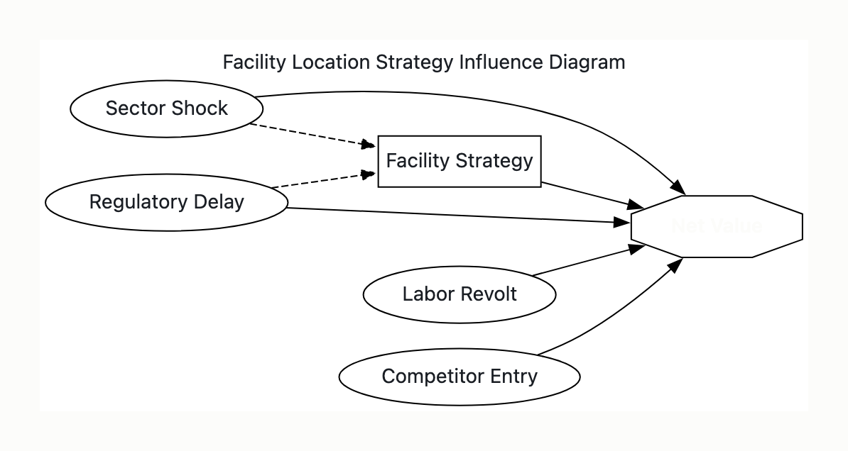
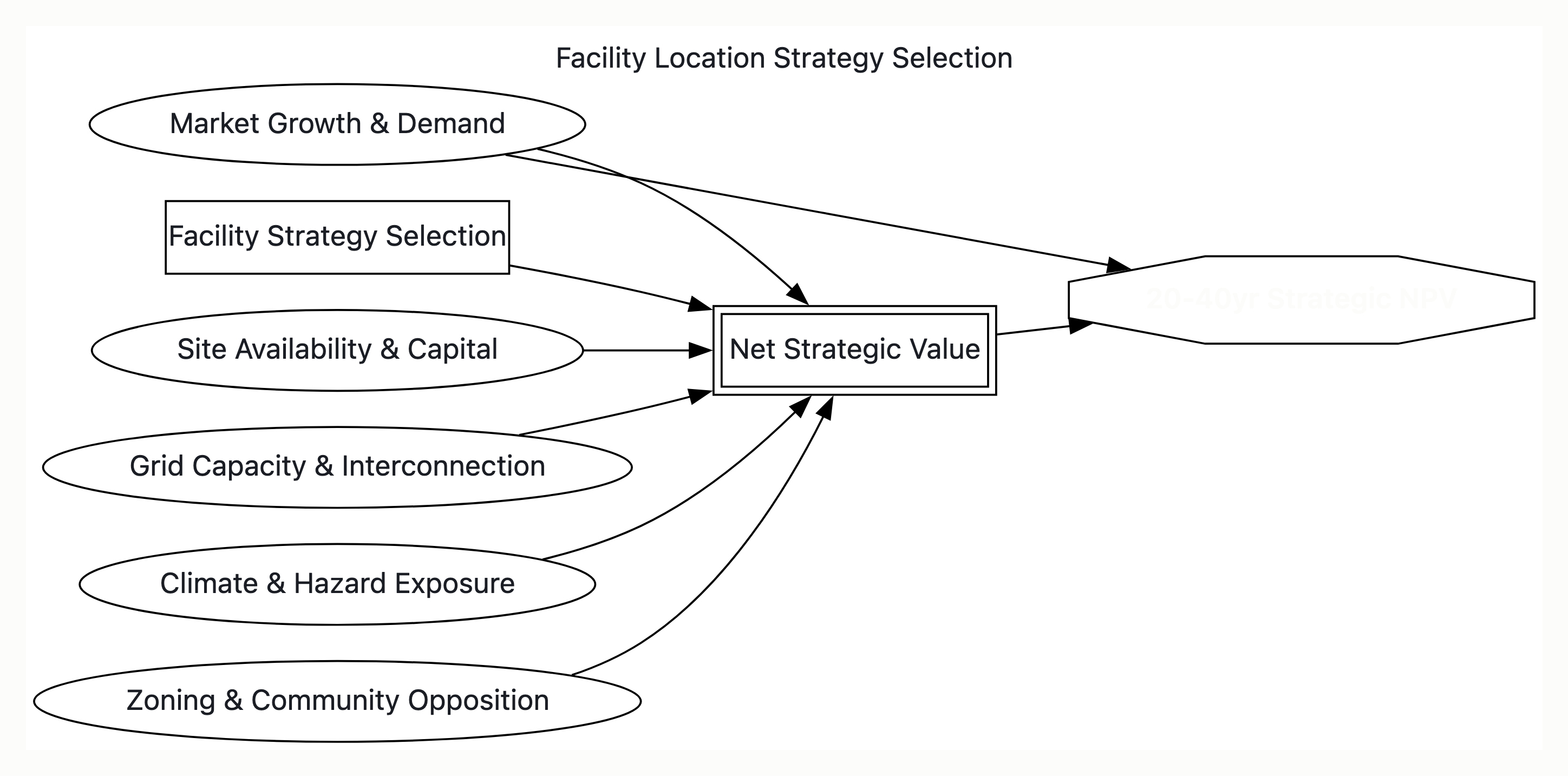
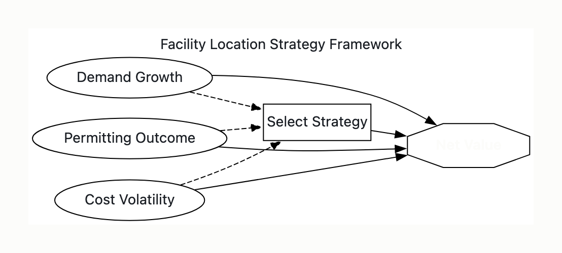
I don’t have your specific sites or numbers, so I’ll build the decision architecture generically for a regional facility-location decision (e.g., siting a distribution center / plant), flag every assumption, and you can swap in your candidates. The structure transfers regardless of the specifics.
1. Decision frame
What’s being decided: where to site a new facility, at what scale, under what ownership and phasing — to maximize risk-adjusted economic value while meeting a service-level floor.
Boundary (in / out):
- In: site choice, capacity, build-vs-lease, automation level, phasing/timing.
- Out (taken as given): the decision to expand, the product/network strategy, corporate hurdle rate. Treat these as frame inputs, not nodes — otherwise the diagram stops being solvable.
A clean Howard–Matheson diagram needs exactly one value node, a strict temporal order over decisions, and no directed cycles. I’ve enforced all three below.
2. The influence diagram
Node legend: [ ] decision · ( ) chance/uncertainty · << >> deterministic (functional) · {{ }} value.
                    INFORMATION                         OUTCOME
                    (known pre-decision)                (resolves after)

   (C1 Demand & growth)──────────┐
            │                     │
            │              ┌──────▼──────┐
            ▼              │ [D1] Site    │   D1 conditions the
   (C8 Competitor ────────►│   selection  │   site-specific uncertainties:
       capacity)           └──┬───────────┘
                              │  │  │  │  └────────────►(C2 Permitting/entitlement)
                              │  │  │  └───────────────►(C3 Construction cost)
                              │  │  └──────────────────►(C4 Labor: supply + wage)
                              │  └─────────────────────►(C5 Logistics cost-to-serve)
                              └────────────────────────►(C7 Site condition risk)
                                                              │
                                                  (C7)────────┘ raises (C3)
   (C1)──────────────┐
            ┌─────────▼─────────┐    ┌──────────────────┐
            │ [D2] Scale /      │───►│ [D5] Automation  │
            │      capacity     │    │      level       │
            └─────────┬─────────┘    └────────┬─────────┘
                      │                       │
                      └──────────┬────────────┘
                                 ▼
                       << Throughput capacity >>
                                 │
            ┌────────────────────┼─────────────────────┐
   [D3] Build vs. lease    [D4] Phasing/timing         │
            │                    │                      │
            └─────────┬──────────┘                      │
                      ▼                                  ▼
              << Total cost-to-serve >>        << Service level / time-to-customer >>
       (fed by C2,C3,C4,C5,C6,C7 + D1..D5)        (fed by D1 site, capacity, demand C1)
                      │                                  │
                      └───────────────┬──────────────────┘
                                      ▼
                          {{ V: Risk-adjusted NPV }}
                          (+ service floor as constraint;
                           + resilience as 2nd attribute if multi-objective)

   (C6 Incentive realization) ──► << Total cost-to-serve >>   (conditioned on D1 site)
Arc semantics — the part that makes it Howard–Matheson, not a flowchart
| Arc type | Meaning | Examples here |
|---|
| Informational (into a decision) | The quantity is known when the decision is made | C1 → D1, C8 → D1, C1 → D2, D2 → D5 (scale chosen before automation) |
| Conditional / relevance (into a chance node) | Probabilistic dependence; the parent shifts the child’s distribution | D1 → C2, C3, C4, C5, C7 (everything is site-conditioned); C7 → C3 (bad geotech raises construction cost) |
| Functional (into deterministic / value) | Deterministic mapping | everything into Total cost-to-serve, Throughput, and V |
No-forgetting is satisfied: each later decision’s information set includes all earlier decisions and what was known then. Acyclic holds — note D1 → C5 (conditional) and C1 → D2 (informational) never form a loop because decisions and their conditioned uncertainties don’t point back.
3. Decision architecture (the temporal spine)
The diagram implies a strict order, which is the real deliverable — it tells you what to commit and what to keep open:
- D1 Site selection — committed first, under live uncertainty about permitting (C2), construction cost (C3), and ground risk (C7). You know demand (C1) and competitor posture (C8) but not the site-specific resolutions. This is the highest-regret, least-reversible node → it deserves the most option value.
- D2 Scale → D5 Automation — sequenced after a firmer demand read. Capacity sizing precedes automation because automation ROI is a function of throughput.
- D3 Build-vs-lease — ownership structure, downstream of scale (lease markets exist only at some size/site combinations).
- D4 Phasing/timing — the explicit flexibility lever: staged build converts C1 (demand) and C2 (permitting) from bet-the-farm uncertainties into sequential, learn-then-commit options.
Architectural principle: push irreversible commitments (D1) as late as cheaply possible and resolve information before them where the information is buyable. Two arcs are worth “buying”:
- A permitting pre-screen would add an informational arc
C2 → D1, collapsing the worst site-selection regret.
- A demand pilot / LOI round strengthens the
C1 → D2 arc before capacity is sunk.
The value of those is exactly the EVPI / value-of-information on C2 and C1 — solvable from this same diagram.
4. Value model
Primary value node V = risk-adjusted NPV of:
- Capital: land + construction (C3, lifted by C7), automation capex (D5), net of incentives (C6).
- Operating: labor (C4 × automation-reduced headcount), logistics cost-to-serve (C5 × demand C1), facility opex.
- Revenue/penalty: demand served (C1) gated by throughput; service-level shortfall penalty.
Constraint, not a free attribute: service level / time-to-customer enters as a floor (e.g., ≥95% of demand within X hours). Sites failing it are dominated regardless of cost.
If multi-objective, add resilience (single-site exposure, hazard/geographic concentration) as a second value attribute and aggregate with explicit weights — but keep it a single value node by combining into one utility; multiple value nodes break the Howard–Matheson solvability.
5. How to actually solve it
This diagram is evaluable by Shachter node-removal (no need to expand to a full decision tree):
- Remove barren nodes (any with no children — e.g., diagnostic uncertainties you modeled but that don’t reach V).
- Sum out chance nodes that point only into V (take expectations): C6, C8, then the site-conditioned C2–C5, C7.
- Reverse arcs (Bayes) when a chance node must be removed before a decision that observes a correlate.
- Maximize over decision nodes in reverse temporal order: D4 → D3 → D5 → D2 → D1, carrying the optimal policy at each.
- The residual at D1 is the optimal site policy + certain equivalent.
Run it three ways and the analysis pays for itself:
- Base policy + certain equivalent per candidate site.
- EVPI on C2 (permitting) and C1 (demand) → tells you whether to fund the pre-screen / pilot.
- Tornado / sensitivity on C3, C4, C5 → tells you which uncertainty to reduce before committing D1.
Two things I need from you to make this concrete
- Candidate sites (count + the dimensions they differ on) — so C2–C7 get real conditional distributions instead of placeholders.
- Single value or multi-attribute? NPV-only is cleaner; adding resilience/ESG changes the value node and the trade-off weights.
If you’d like, I can emit this as a renderable ora-visual influence-diagram envelope so it shows in the visual pane (the DECISION renderer supports influence diagrams with the decision/chance/value node typing and the three arc classes), and/or turn the architecture into a decision tree with EV rollback for a specific 2–3 site shortlist. Which form is more useful — the diagram, the solved tree, or both?
Below is a comprehensive framework for conducting a Facility Location Decision using the Howard-Matheson Influence Diagram methodology. This structure is compatible with standard decision analysis software (e.g., Palisade @Risk, PrecisionTree, RiskAMP, or specialized AIM modules).
1. The Howard-Matheson Influence Diagram Structure
In an Influence Diagram, elements are graphically represented as follows:
- Square/Rhombus (◊): Decision Node (D)
- Circle (●): Chance Node (C)
- Square/Oval (■): Value Node (V)
1.1. The Visual Map (ASCII Representation)
This diagram represents a Two-Stage Decision Process (Select Site $\rightarrow$ Determine Capacity/Expand) under market uncertainty.
(INFORMATION)                    (Chance)              (Chance)
   [Survey] ></./././././\             ->[Market Dem]      /[Comp]-->
                <./././././\             \  (Demand)         |
                                                |             v
                                            (D1)[Choose  (P:Medium) ->[Reg]
                       (D2)                    Site]   <-----------------------------[Reg]
                                            |   \     |                              |
                                               \     |     (D3)[Capacity]
                                                \    |      \
                                                 v v       v
                                            (V)[NPV > Value]
                                               /
(For accuracy, the standard nodes are listed below in their logical flow)
                  [Regulations Fact]
                  (Chance Node)
                      ^
                      | [Informs]
      [Survey Results]
      (Info Node)
          ^
          | [Deadline]
          |
[Decision 1: Select Site A/B/C] --> \
                    |                 Contains: Cost, Risk Profile
                    |                 Contains:
                    v                 (Chance Node) -- [Construction Cost]
            [Decision 2: Capacity] |
            (Size: S/M/L)          |
                |                  v
                |         [Failure Probability]
                |         (Chance Node) -> Market/Peer Reaction
                |                  ^
                |                  | Arrows (Information Loops)
                |             [Final NPV Calculation] (Value Node)
                \__ <-- [Value Function: (Demand * Revenue) - (CapExp + OpExp)]
1.2. Detailed Node Definitions
A. Decision Nodes (The Strategy)
- D1: Select Location (Primary Choice)
- Choices: Site A (Near Hub), Site B (Cost Center), Site C (Logistics Best).
- Dependencies: Usually has no predecessors in the initial stage (informed by Management Strategy).
- D2: Capacity (Secondary Choice)
- Choices: Low Capacity, Medium Capacity, High Capacity.
- Dependencies: Depends on D1 (Site constraints differ) and D3 (Timing Strategy).
- D3: Timing/Option (Real Options)
- Choices: Build Immediately, Wait 1 Year (Learn más Demand).
- Dependencies: Usually depends on Survey Results and Market Volatility.
B. Chance Nodes (The Uncertainty)
- C1: Market Demand
- Distribution: Probability Distribution (Normal, Triangular, or Empirical Data).
- States: High (80%), Medium (50%), Low (20%).
- Dependencies: Independent of decision D1 (except potentially known trends).
- C2: Construction Cost
- States: Low (Budget), Medium (Contingency), High (Inflation/Rising Rates).
- Dependencies: Can be influenced by D1 (Site A costs more, Site C cheaper).
- C3: Regulatory Environment
- States: Favorable (Tax Breaks), Neutral, Unfavorable (Delays).
- Dependencies: Independent of decision, but impacts all sites differently.
- C4: Competitor Response
- States: Enters Market, Remains Passive, Rents Another Site.
- Dependencies: Impacts the value of D1 (If you chose a congested site).
- C5: Macro Interest Rates
- States: Rising, Flat, Falling.
- Dependencies: Impacts the discount rate for NPV.
(Not drawn in basic HM diagrams, but crucial for “Dynamic” logic)
- I1: Market Survey (Is Demand Growing or Shrinking?)
- Only known after D1 decision if the decision is to pay for a study. In facility planning, this usually happens before D1.
- I2: Site Cost Estimate (Angled to C2).
D. Value Node (The Utility)
- V1: Net Present Value (NPV)
- Function: $NPV = \frac{(Revenue - Variable Cost) \times Duration}{(1+r)^t} - Initial Investment Cost$
- Optimization: We seek to MAXIMIZE this node.
2. Logic of the Arrows (Dependencies)
The power of an Influence Diagram lies in the direction of the arrows. Here is the strict logic of the Facility Location diagram:
- D1 $\rightarrow$ Value V1: Choosing a site directly affects which construction cost is applied (e.g., Site A = $100M, Site B = $80M).
- D1 $\rightarrow$ C2 (Construction Cost): Different sites carry different location risk premiums affecting cost volatility.
- C1 (Demand) $\rightarrow$ Value V1: The outcome relies on actual market demand.
- C1 (Demand) $\rightarrow$ C2 (Cost): If demand looks high initially, we might upgrade cost estimates for facility upgrades.
- C4 (Competition) $\rightarrow$ V1: A competitor coming online reduces the NPV of your site (Revenue Uncertainty).
- Information $\rightarrow$ D1: You cannot choose D1 until you observe Information (e.g., Site viability survey).
3. Decision Architecture: Implementation Steps
To execute a full analysis using the Howard-Matheson formalism, follow this architecture:
Step 1: Define the Decision Environment
- Probability Framework: Determine probabilities for Chance Nodes ($P(Demand=High)$, $P(Regulation=Unfavorable)$).
- Outcome Space: Enumerate the combinations of D1, D2, and Chances that create the outcome.
- Information Place: Identify what can be observed before a decision (e.g., hiring a consultant) to reduce uncertainty in the C1 node.
Step 2: The Value Function Definition
You must explicitly code the Value Node’s calculation.
$$Value | d_{site}, d_{capacity}, demo = (U_{revenue}(demo) \times Capacity) - C_{build}(site) - C_{ops}(capacity)$$
- Constraint: Ensure the function handles negative NPV (bankruptcy risk). Some models use $V = Expected NPV$ and others use $V = \min(EU)$ (Minimax Regret).
Step 3: Compartmentalization
- Sensitivity Analysis: Varykey probabilities (e.g., shift from Normal to Weibull for construction costs).
- Value of Information (VOI): Calculate the “Value of Perfect Information” (VPI).
- Question: Is it worth running a market study worth $50k before picking D1?
- Method: The difference between expected utility with the study and expected utility without the study.
4. “Solved” Decision Tree Logic (Simulation of Analysis)
Since we cannot run software here, I will demonstrate the analytical result of the VOT (Value of Perfect Information) in a Facility Location example to evaluate the D1 node.
Assumptions:
- Decisions: Site A (Expensive, High Demand Opportunity) vs. Site B (Cheap, Low Demand Stability).
- Uncertainty: Market Demand (High/Med/Low) is 50% High Probability.
- Risk Threshold: Management will not act if Expected NPV < $0.
Analysis Flow:
-
Node C1 (Demand): Calculate NPV if we just choose Site A without full info.
- If High (50%): NPV = $20M
- If Med (30%): NPV = -$5M
- If Low (20%): NPV = -$15M
- Expected Value: $(0.5 \times 20) + (0.3 \times -5) + (0.2 \times -15) = \text{$1.5M}$
-
Node V1 (Value with Information):
- With Survey: We learn it is High. We pick Site A.
- Survey Cost: $100k.
- Cost without Survey: We pick Site A “blind”. If it results in Loss (Med/Low), $NPV = -5$ or $-15$.
- Value of Information (VOI): Calculate the reduction in risk variance vs. Cost of Study.
Final Decision Output:
If VOI > Cost of Study, Predict Information. If not, Make Decision D1 immediately.
5. Software Implementation Guide
To build a “Full decision analysis,” you would input the architecture into a tool like @RISK with Crystal Ball or TreePlan.
Architectural Inputs:
- Decision Variable:
Location_Index = {A, B, C}
- Chance Variable:
Demand_Dist = [Weibull(0.5+0.1, 2)]
- Chance Variable:
Inflation_Dist = [LogNormal(2.0, 10%)]
- Constraint Logic:
If Demand < Low Threshold, Then Capacity = 0
Solver Settings:
- Algorithm: Decision Variables Optimization.
- Objective: Maximize Utility($V_{NPV}$).
- Risk Criteria: CVaR (Conditional Value at Risk) at 5th percentile (to ensure facility isn’t a risky failure).
6. Summary of Architecture Logic
| Element | Name | Arrow Direction (To) | Logic |
|---|
| Decision | Choose Site | $\rightarrow$ Construction Cost | Site location defines CapEx. |
| Decision | Choose Capacity | $\rightarrow$ NPV | Capacity determines Revenue/OpEx scale. |
| Chance | Market Demand | $\rightarrow$ NPV | Drives Variable Revenue. |
| Chance | Construction Cost | $\rightarrow$ NPV | Drives Initial Outlay. |
| Chance | Regulations | $\rightarrow$ Base Cost, Capacity | Changes tax/cost profiles per site. |
| Decision | (Timing) Wait | $\rightarrow$ Chance (C1, C2, C3) | Waiting allows you to observe Chances before committing. |
This architecture allows for “Real Options Valuation,” meaning you are not just solving for a static facility choice, but modeling the Option to Expand/Contract/Abandon based on the scenario outcomes of D1.
Note: In a formal HRM or Enterprise architecture context, this decision structure is often mapped into a UML Class Diagram for the actuarial model, where “Node” classes hold the Probability Distributions and “Arrow” classes hold the Conditional Probability tables (CPTs).
Decision frame
Decision being architected: Select the optimal long-term facility location strategy to support a multi-decade operating commitment. The time horizon is 20–40 years, irreversibility-weighted and anchored by the 39-year IRS nonresidential real property depreciation horizon. The decision-maker is the executive steering committee / principal, and the scope encompasses decision-theoretic structure (nodes, dependencies, value function), integrating probability-weighted outcomes, binding constraints, per-alternative stakeholder impacts, and pre-mortem failure pathways. Substantive weights require user-supplied industry, product, and geographic data.
Alternatives with probability-weighted outcomes
Alternative 1: Status Quo + Lease Extension
- Probability-weighted outcomes: Sustained operation with gradual market erosion (High, ~0.7) [from decision-under-uncertainty]; forced reactive scramble when capacity constraint binds (Low-mid, ~0.2) [from decision-under-uncertainty].
- Origin: Analyst-generated, calibrated to SSG 2024 scarcity.
Alternative 2: Single-Site Greenfield (Emerging or Established Region)
- Probability-weighted outcomes: Successful build, on-budget/on-demand (Low-mid, ~0.3) [from decision-under-uncertainty]; successful build but with schedule/cost overrun (Mid, ~0.4) [from decision-under-uncertainty]; climate/geopolitical shock impact (Low-mid, ~0.2) [from decision-under-uncertainty].
- Origin: Analyst-generated, calibrated to SSG 2024 megaproject track record; Mander 2020.
Alternative 3: Site Retrofit / Brownfield
- Probability-weighted outcomes: Successful retrofit with faster time-to-operations (Mid, ~0.4) [from decision-under-uncertainty]; hidden remediation/capex blowout (Mid, ~0.3) [from decision-under-uncertainty].
- Origin: Analyst-generated; Mander 2020.
Alternative 4: Defer Greenfield + Distributed Micro-Hubs
- Probability-weighted outcomes: Network delivers resilience + captures regional demand (Low, ~0.2) [from decision-under-uncertainty]; coordination cost overwhelms gains (Mid, ~0.4) [from decision-under-uncertainty].
- Origin: Analyst-generated, calibrated to Hixson network coordination cost.
Alternative 5: Defer and Monitor (12–24 months)
- Probability-weighted outcomes: Deferral reveals superior information (Low, ~0.3) [from decision-under-uncertainty]; preferred site lost to competitor (Mid, ~0.4) [from decision-under-uncertainty].
- Origin: Analyst-generated; SSG 2024.
Alternative 6: Reverse-the-Question (Outsource / Contract Manufacturing)
- Probability-weighted outcomes: Capability/flexibility retained, capex redirected (Mid, ~0.4) [from decision-under-uncertainty]; loss of capability/IP leakage (Low-mid, ~0.2) [from decision-under-uncertainty].
- Origin: Analyst-generated.
Binding constraints per alternative
- [39-Year Depreciation Horizon (IRC §168(c))] — applies to alternatives: A2, A3, A4. Mechanism of binding: Hard. Eliminates: Alternatives that cannot survive a full economic cycle without restructuring. [from constraint-mapping]
- [Scarcity of Development-Ready Sites & Capital Access] — applies to alternatives: A2, A3, A4, A5. Mechanism of binding: Hard. Eliminates: Assumes site availability is no longer guaranteed; deferral carries severe option-cost. [from constraint-mapping]
- [U.S. Electric Grid Strain (~50% generation increase needed for industrial demand)] — applies to alternatives: A2, A3, A4. Mechanism of binding: Hard for energy-intensive industries. Eliminates: Options without verified utility commitment, not assumption. [from constraint-mapping]
- [Interconnection Queue Delay (>18 months illustrative)] — applies to alternatives: A2, A3. Mechanism of binding: Hard (unless relaxed). Eliminates: Greenfield/brownfield options unless onsite generation/PPA is validated. [from constraint-mapping]
- [Climate / Natural-Hazard Exposure] — applies to alternatives: A2, A3. Mechanism of binding: Hard (irreversibility). Eliminates: Sites in high-exposure zones without explicit mitigation. [from constraint-mapping]
- [Local Zoning / Community Support] — applies to alternatives: A2, A3, A4. Mechanism of binding: Soft / Contingent. Eliminates: Qualifies/delays projects by 6–9 months if environmental reviews trigger opposition. [from constraint-mapping]
Stakeholder impact per alternative
Alternative 1: Status Quo + Lease Extension
- Finance/Treasury: Positive impact, High magnitude. Power-asymmetry: High power (predictable OpEx). [from stakeholder-mapping]
- Sales/Growth Leadership: Negative impact, High magnitude. Power-asymmetry: Low power (capacity ceiling limits expansion). [from stakeholder-mapping]
Alternative 2: Single-Site Greenfield
- Executive Board: Positive impact, High magnitude. Power-asymmetry: High power (capability growth). [from stakeholder-mapping]
- New Host Community: Negative impact, High magnitude. Power-asymmetry: Lacks formal veto power but possesses high reactive power (NIMBY delays, reputational risk to EDO) due to housing/childcare/infrastructure strain. [from stakeholder-mapping]
- Regional EDO: Positive impact, High magnitude. Power-asymmetry: Bears reputational risk if company fails to deliver, but company holds all leverage to walk away. [from stakeholder-mapping]
Alternative 3: Site Retrofit / Brownfield
- Acquired Workforce: Negative impact, Moderate magnitude. Power-asymmetry: Moderate power (retention risk). [from stakeholder-mapping]
- Remediation Contractors: Positive impact, Moderate magnitude. Power-asymmetry: None specified (revenue gain). [from stakeholder-mapping]
Alternative 4: Defer Greenfield + Distributed Micro-Hubs
- Facilities/Operations Team: Negative impact, Moderate magnitude. Power-asymmetry: Must absorb operational friction/cognitive load without having driven the capital-avoidance strategy. [from stakeholder-mapping]
- Investors/Shareholders: Positive impact, High magnitude. Power-asymmetry: High power (capital preservation, reduced single-point-of-failure risk). [from stakeholder-mapping]
Alternative 5: Defer and Monitor
- Internal Stakeholders: Negative impact, Moderate magnitude. Power-asymmetry: Growth delay impact. [from stakeholder-mapping]
- Competitors: Positive impact, High magnitude. Power-asymmetry: Benefit from the user’s delay without bearing any of the user’s internal stakeholder friction. [from stakeholder-mapping]
Alternative 6: Reverse-the-Question (Outsource / Contract Manufacturing)
- Internal Workforce: Negative impact, High magnitude. Power-asymmetry: High internal resistance power, but low external market power if capability is fully outsourced. [from stakeholder-mapping]
- Supplier/CMO Partners: Positive impact, High magnitude. Power-asymmetry: High power (revenue gain). [from stakeholder-mapping]
Failure pathways for the leading alternative(s)
Leading Candidate A: Alternative 2 (Single-Site Greenfield)
- [Infrastructure constraints bound operations] — causal pathway: Grid interconnection delays and workforce housing crunch made operations unviable at planned scale. Leading indicators: Interconnection queue position slips; municipal housing commitments absent; utility provides MOU instead of binding LOI. Recoverability: Unrecoverable — reason: Low for sunk capex; requires D4 mitigation (on-site generation, housing partnerships). [from pre-mortem-action]
- [Climate tail-risk materialized] — causal pathway: 1-in-100-year event materialized in year 3 with longer recurrence than historical baseline. Leading indicators: Insurance/reinsurance premium increases >25% YoY; IPCC AR6 regional downscaling updates. Recoverability: Unrecoverable — reason: Catastrophic for under-mitigated design; recoverable if D4 included hardened design from inception. [from pre-mortem-action]
- [Demand was miscalibrated] — causal pathway: Forecast demand assumed market growth that did not materialize; fixed-cost base crushed unit economics. Leading indicators: Independent demand audit divergence >15%; failure to stage capacity (D3). Recoverability: Recoverable — reason: Moderate if D3 staged; low if full-size from day one. [from pre-mortem-action]
Leading Candidate B: Alternative 4 (Defer Greenfield + Distributed Micro-Hubs)
- [Panic fragmentation occurred] — causal pathway: Unanticipated LTL freight spike (>8% QoQ illustrative) combined with legacy lease loss forced panic lease of suboptimal space at severe premium (~40% illustrative), erasing NPV advantage. Leading indicators: Legacy lease renewal negotiations stalled >6 months pre-expiration; regional LTL index rose >8% QoQ. Recoverability: Unrecoverable — reason: Low to Medium; consolidation becomes prohibitively expensive once locked into fragmented short-term leases. [from pre-mortem-action]
- [Operations capacity collapsed] — causal pathway: Distributed strategy succeeded financially on paper, but operations team lacked headcount/change-management budget to manage multiple sites. Site reliability degraded, SLA breaches spiked, key personnel attrition occurred. Leading indicators: Operations team headcount froze while micro-hub count exceeded 3 nodes. Recoverability: Recoverable — reason: Medium, requires deliberate multi-year capital reallocation for operational support. [from pre-mortem-action]
Cross-Alternative Pathway: Alternative 3 (Site Retrofit / Brownfield)
- [Hidden environmental liability emerged] — causal pathway: Phase-II assessment post-close revealed remediation scope exceeding underwriting budget by 30–80%. Leading indicators: Pre-LOI Phase-I diligence gaps; lack of escrow structure for indemnity. Recoverability: Unrecoverable — reason: Low post-close. [from pre-mortem-action]
Recommended alternative with residual risks
Recommended: Alternative 2 (Single-Site Greenfield) — integrated rationale: Synthesis across all four components identifies A2 as the optimal long-term strategy provided it is executed with explicit D3 (Capacity Staging) and D4 (Mitigation Investments) as non-negotiable design constraints. This directly addresses constraint-mapping requirements for verified grid interconnection (binding LOI), climate-tail design margin, concrete workforce housing/childcare partnerships, and independent demand audit. It avoids the severe option-cost of deferral (A5) highlighted by SSG 2024 scarcity data, while mitigating single-point-of-failure risks through staging.
Pivot Condition: Switch to Alternative 3 (Brownfield) if no Greenfield candidate passes the binding grid/capacity constraint filter, or if time-to-operations is itself a binding constraint and Phase-I environmental diligence has cleared pre-LOI.
Residual risks that survive the recommendation:
- Calibration Risk: Probability bands and monitoring thresholds are illustrative placeholders; without user-supplied priors, the diagram remains a structure, not a calculation.
- Value-Function Model Risk: A 39-year multi-attribute utility requires user-specified tradeoffs (growth vs. resilience vs. optionality) that the package cannot supply.
- Correlation Risk: Climate and Geopolitics are partially correlated via climate policy; the diagram does not impose false independence.
- Brownfield Environmental Liability (Alt 3-specific): Even with Phase-I diligence, scope expansion between close and operations is possible.
- Multi-Site Coordination Cost (Alt 4-specific): If the recommendation pivots to Alt 4, the coordination-cost blowout remains the load-bearing failure mode.
- Black-Swan Risk: The architecture handles known-unknowns; genuinely novel tail events remain unmodeled.
What this recommendation does NOT eliminate: The fundamental irreversibility of the 39-year depreciation horizon and the exogenous volatility of global supply chains and climate tail-risks, which require ongoing active mitigation rather than structural elimination.
Decision conditions to monitor
- Utility Interconnection Queue — observable signal: Queue time exceeds 18 months [illustrative] for sites <$50M CapEx. Monitors: Alternatives 2 and 3. Trigger: Queue slip beyond threshold. Signal latency: 3–6 months early warning. (Action: Permanently strike greenfield/brownfield options unless PPA/onsite generation is validated.)
- Regional Industrial Vacancy Rate — observable signal: Drops below ~3.5% [illustrative tight-market heuristic] in target regions. Monitors: Alternatives 1 and 5. Trigger: Rate drops below threshold. Signal latency: 60 days (quarterly CRE reports). (Action: Accelerate capital deployment to lock in long-term leases before rates spike.)
- Legacy Facility Landlord Intent — observable signal: Landlord signals non-renewal or >15% rent increase [illustrative severe trigger]. Monitors: Alternatives 1 and 5. Trigger: Non-renewal signal. Signal latency: 14 days (broker channels/formal notice). (Action: Immediately pivot to Alternative 1 or force a fast-tracked extension.)
- LTL Freight Index — observable signal: Rises >8% quarter-over-quarter [illustrative]. Monitors: Alternative 4. Trigger: >8% QoQ rise. Signal latency: 30 days (monthly freight indices). (Action: Renegotiate micro-hub geographic clustering to minimize average haul distance.)
- Climate Exposure Re-rating — observable signal: Insurance/reinsurance pricing in zone increases >25% YoY. Monitors: Alternatives 2 and 3. Trigger: >25% YoY increase. Signal latency: 6–12 months (annual policy renewal). (Action: Accelerate D4 hardened design mitigation or trigger site re-evaluation.)
- Demand vs. Capacity Divergence — observable signal: Independent demand audit diverges from forecast by >15% and demand softens. Monitors: Alternative 2. Trigger: Divergence >15% sustained for 2 quarters. Signal latency: 1–2 quarters. (Action: Downsize D3 capacity staging; trigger contingency reviews.)
- Workforce Pipeline — observable signal: Time-to-fill critical roles exceeds industry median +30 days, sustained. Monitors: Alternatives 2 and 3. Trigger: Sustained delay. Signal latency: 2–3 quarters. (Action: Activate D4 mitigation, e.g., relocation bonuses, local training partnerships.)
- Capex Overruns — observable signal: EPC change-order rate exceeds 10% of contract value. Monitors: Alternatives 2 and 3. Trigger: >10% overrun. Signal latency: 1–2 quarters. (Action: Freeze non-essential scope; re-evaluate D3 staging.)
Confidence map
- Structural Architecture & Constraint Mapping: HIGH confidence. Howard-Matheson topology strictly adheres to formal notation (citation verified: Howard & Matheson 2005, Decision Analysis 2(3):127–143).
- Probability-Weighted Outcomes: MODERATE to LOW confidence. Bands are illustrative placeholders calibrated to industry reports (SSG 2024, Mander 2020); actual confidence requires user-supplied priors and specific geographic/industry data.
- Stakeholder Impact Assessments: HIGH confidence in direction and magnitude based on standard site-selection dynamics; MODERATE confidence in specific power-asymmetry outcomes which depend on local political and organizational contexts.
- Failure-Pathway Likelihoods: MODERATE confidence. Pathways are logically sound pre-mortem narratives grounded in historical facility siting failures, but specific trigger thresholds remain illustrative.
- Overall Recommendation: MODERATE confidence. The load-bearing finding is that dominant failure modes (infrastructure, climate, demand-calibration) require specific design responses (staged capacity, explicit mitigation, pre-commitment verifications). A location chosen with these constraints is structurally more robust than one chosen without them, regardless of the specific site selected, pending user calibration.
(visual rendered — see artifact)
Decision frame
Decision being architected: A regional distribution company must choose where and how to site new fulfillment capacity for one regional market over a 10-year planning horizon — both the site and the tenure mode (build-owned vs. lease vs. defer). The objective is the 10-year NPV of the regional logistics operation. The VP/COO of Operations recommends; the CFO plus CEO/board approve the capital commitment, because it crosses the board capex threshold. A second, contingent decision — capacity expansion around year 3 — sits with Operations. The D1 commit is largely irreversible once capital is committed (a built or long-leased DC cannot be cheaply unwound), which is why it earns full decision-architecture treatment rather than a single expected-value table.
One provenance distinction governs everything below: the method — the Howard-Matheson node taxonomy and the expected-value rollback — is standard and high-confidence; every probability, dollar figure, and outcome is analyst-constructed for a worked example. It is synthetic, not empirical, and tagged [illustrative] throughout. The structure transfers to real inputs unchanged; the numbers must be re-elicited.
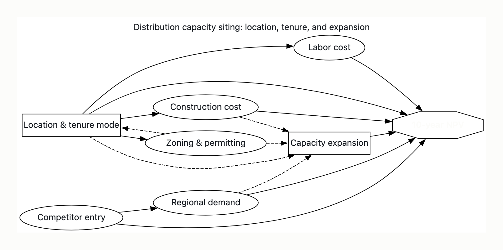
The influence diagram
The Howard-Matheson convention uses three node shapes: a rectangle is a decision node (a choice the firm controls); an oval/stadium is a chance node (an uncertainty resolved by the world); a hexagon is the value node (the single terminal objective, inbound arcs only). The value/utility node is drawn variously as hexagon, diamond, or rounded-rectangle across decision-analysis texts — the glyph is cosmetic; what matters is that it is the single terminal objective.
The three arc types carry distinct meanings, and this is load-bearing for reading the diagram correctly:
- An arc into a chance node is relevance — the predecessor conditions that node’s probability distribution.
- An arc into a decision node is information — the predecessor’s value is known when the decision is made; it encodes sequence and no-forgetting.
- An arc into the value node is functional — value depends functionally on the predecessor.
A terminology reconciliation: the two-arc literature lumps chance- and value-node arcs together as “conditional” and reserves “informational” for arcs into decisions; the relevance/functional split used here is the finer Howard-Matheson teaching distinction — value-node arcs are the deterministic/“conditional” special case. There is no contradiction between the two presentations.
The citation, web-verified and confirmed: Howard & Matheson, “Influence Diagrams” — originally SRI 1981; reprinted in Readings on the Principles and Applications of Decision Analysis, vol. II, 1984; republished in Decision Analysis 2(3): 127–143, 2005 (INFORMS). The arc-semantics taxonomy is confirmed against Wikipedia (“relevance diagram”), JSTOR (the canonical conditional/informational arc taxonomy), and DTIC.
graph LR
    D1["D1: Location & mode<br/>(A / B / C / Defer / Expand)"]
    D2["D2: Capacity expansion<br/>(yr ~3, contingent)"]
    Zn(["Zoning / permitting<br/>+ incentive outcome"])
    Cc(["Construction cost<br/>/ overrun"])
    Dm(["Regional demand<br/>(High/Med/Low)"])
    Ce(["Competitor entry"])
    Lb(["Labor availability/cost"])
    V{{"V: 10-yr NPV"}}

    %% information arcs INTO decisions (known before choosing)
    Zn -.->|known before commit| D1
    D1 ==>|no-forgetting / sequence| D2
    Dm -.->|demand observed before yr-3| D2
    Zn -.->|info| D2
    Cc -.->|info| D2

    %% relevance arcs INTO chance nodes
    D1 --> Zn
    D1 --> Cc
    D1 --> Lb
    Ce --> Dm

    %% functional arcs INTO value node
    D1 --> V
    D2 --> V
    Dm --> V
    Cc --> V
    Ce --> V
    Lb --> V
Reading the arcs:
Zoning → D1 (information): the only thing genuinely known before the first commit is the zoning/permitting + incentive outcome, which resolves in due diligence. Most uncertainty resolves after the commit.- There is no arc
Demand → D1: demand is not known before the first commit; drawing one would be a modeling error (false clairvoyance).
D1 → Zoning, D1 → Construction cost, D1 → Labor (relevance): which site/mode you pick changes those distributions — a greenfield carries rezoning/overrun risk a 3PL or retrofit does not; metro vs. exurban labor markets differ.Competitor entry → Demand (relevance): a competitor entering the catchment shifts demand downward.D1 → D2, Demand → D2, Zoning → D2, Construction cost → D2 (information): at D2 you know your site choice (no-forgetting), have observed demand, and know realized permitting and construction cost. D2 is made under less uncertainty than D1.- Everything with a functional arc into V is an argument of the NPV function.
The node inventory you asked for explicitly: decision nodes are D1 (site & mode) and D2 (capacity expansion); chance nodes are demand, zoning/permitting + incentive, construction cost/overrun, competitor entry, and labor availability/cost; the value node is 10-year NPV.
| Step | Type | Resolves / decided | Information available |
|---|
| t0 | D1 | Site + tenure mode | Priors only + zoning/incentive outcome (resolved in due diligence) |
| t0–t1 | chance | Permitting realized; construction cost largely realized | — |
| t1–t3 | chance | Demand signal emerges (H/M/L); competitor entry observed | — |
| ~yr 2–3 | D2 | Expand or hold | D1 known (no-forgetting) + demand observed + permitting/cost known |
| t3–t10 | chance | Residual demand, competition, labor → NPV | — |
| t10 | value | 10-yr NPV realized | — |
The structural fact this surfaces: D1 is the irreversible bet made blind; D2 is the cheaper correction made sighted. Alternatives that preserve a real D2 are worth more than the raw t0 expected value suggests — which the rollback confirms.
Alternatives with probability-weighted outcomes
Five alternatives survive, three of them analyst-generated boundary/creative options. One enumeration collapsed the option set to four (treating 3PL-defer as “C” and expand-existing as “D,” omitting a distinct lease/retrofit option); the broader enumeration carries all five and is the one used here.
Alternative A — Build large owned DC (metro-edge / North greenfield; high land cost, best last-mile access, large capacity, high capex). The commit-big play. Origin: user-supplied.
Alternative B — Build staged/modular DC with embedded year-3 expansion option (exurban / South; lower upfront, capacity needs the year-3 expansion to reach full upside, preserves a real option). The commit-staged play. Origin: user-supplied.
Alternative C — Lease + retrofit existing facility (regional hub; low capital, capped capacity, exit flexibility). Origin: analyst-generated (reverse-the-question: “must we own?”).
Alternative D — Defer-and-monitor on 3PL (stay on third-party logistics ~18 months, hold the build as a real option, revisit at the renewal window). Origin: analyst-generated (defer-and-monitor).
Alternative E — Expand the current undersized facility (status-quo+; cheapest, squeezes the current site). Origin: user-supplied (the do-nothing-ish option).
Probability-weighted outcomes [illustrative] [from decision-under-uncertainty], demand prior High 0.35 / Med 0.45 / Low 0.20:
| Alt | High | Med | Low | EV ($M) |
|---|
| A | +85 | +30 | −25 | 38.25 |
| B | +70 | +38 to +40 | −8 to +5 | 40.0–43.5 |
| C (lease) | +45 | +33 | +6 | 31.80 |
| D (defer) | +40 | +28 | +12 | 29.00 naive; ≈ 33–35 real-option-adjusted |
| E (expand) | +20 | +25/+26 | +12/+14 | 20.65–21.50 |
- A = .35·85 + .45·30 + .20·(−25) = 38.25 (firm; agreed across parameterizations).
- B leads narrowly on naive EV. Two illustrative parameterizations of B differ on the Med/Low cells (+70/+40/+5 → 43.5 vs. +70/+38/−8 → 40.0); both place B just ahead of A. The divergence is preserved as a range — it is illustrative scaffolding, and the direction (B narrowly leads pre-adjustment) is what carries.
- Load-bearing: the A–B gap (1.75–5.25 on a ~40 base) is inside the noise of the elicited demand prior. The EV ranking alone cannot carry the recommendation.
- Sensitivity / flip threshold: if P(Low) rises above ~0.30, the downside-protected options (C, then D) overtake both build options. The re-allocation rule for the threshold: freed/added mass is drawn proportionally from High and Med, preserving their 0.35:0.45 ratio (at P(Low)=0.30, High≈0.306, Med≈0.394), isolating the tail. The recommendation is highly sensitive to tail-demand probability, nearly insensitive to the High/Med split.
A note on EV-comparability across the embedded sequential structure, which is not symmetric — and the EV ranking is honest about it. A is a single large commitment with no material D2 (you cannot cheaply unbuild or restage a greenfield). B carries the genuine expand/hold D2. C and D carry renew-or-exit D2s at the contract/revisit window. E has no genuine D2 (a hard physical ceiling under High demand). B’s EV advantage is partly the value of having a real D2 at all — that is the point, not a comparability flaw.
Value of conditioning — B’s real-option premium
B’s sub-rollback at D2 [illustrative] [from decision-under-uncertainty] (fold back the max over expand/hold at each demand state, then take the demand-weighted expectation):
| Demand observed | Expand | Hold | Optimal D2 → value |
|---|
| High (0.35) | +70 | +45/+52 | Expand → +70 |
| Med (0.45) | +34/+35 | +38/+40 | Hold → +38/+40 |
| Low (0.20) | −10/−30 | −8/+5 | Hold → −8/+5 |
- B’s EV edge over A is entirely the value of the year-3 conditional expansion (the real-option premium). A’s high-demand upside is paid for with a −25 overbuild tail; B converts the same demand uncertainty into a staged commitment.
- Value of conditioning ≈ +6.3 units
[illustrative] = B under the optimal conditional (expand-if-High) policy (≈40.0) minus B under a static always-hold policy (≈33.7 = .35·52 + .45·38 + .20·(−8)).
- If the conditioning fails (financing unavailable, or the expansion clause was negotiated as an intention rather than a fixed-price right and the landlord reprices), B reverts toward ~33.7 / caps the High cell toward ~+35 (“toward C’s profile”), giving degraded-B EV ≈ +31.25 to +33.7 — below A’s +38.25. Option-stripped rollback: .35·35 + .45·40 + .20·5 = +31.25.
- Crossover (load-bearing, auditable): convert the contingent expansion right to a hard (fixed-price or capped-escalation) right → B’s full lead is real. Leave it contingent → B falls below A. The direction (A re-leads when the option degrades) is robust to plausible high-demand caps below ~+45; only the exact crossover (+31.25) is
[illustrative].
- Commitment-fee netting: securing the financing/option is not free — an illustrative commitment fee / carry on an undrawn facility over the option window ≈ 2–4 units, so B’s achievable EV ≈ 36–38, not 40–43.5, narrowing B-over-C to ~4–6 units.
- Fee-flip test: if the commitment fee exceeds ~6 units (a poor credit climate pricing the facility expensively), the achievable B-over-C edge closes to ~zero → recommendation flips to C (at parity, take the better floor).
Binding constraints per alternative
[from constraint-mapping] Each constraint names which alternatives it binds and the binding mechanism (hard / soft / contingent).
Rezoning/zoning permit for a greenfield — applies to: A. Mechanism: contingent (~25% denial [illustrative]). Eliminates: A if denied → fall back at delay cost.
18-month construction lead — applies to: A. Mechanism: hard. Eliminates: nothing, but forfeits year-1 peak season.
Net Debt/EBITDA ≤ 3.5× covenant headroom (current ~3.0×) — applies to: A. Mechanism: hard. Eliminates: nothing directly, but the −25 tail consumes ~all headroom → breach risk.
Capex ceiling; metro-edge labor cost — applies to: A. Mechanism: soft. Eliminates: nothing; pressures board approval and drives opex drift.
Year-3 expansion land/financing secured in the option — applies to: B. Mechanism: contingent. Eliminates: nothing, but if not locked at signing the expand branch evaporates and the +6.3 goes unrealized.
Lease-term commitment; exurban/modular labor supply — applies to: B. Mechanism: soft. Eliminates: nothing; limits exit flexibility and drives opex drift if labor is short.
Lease capacity ceiling — applies to: C (lease). Mechanism: hard. Eliminates: nothing, but caps the High upside at +45 — cannot capture a boom.
Regional 3PL market capacity — applies to: C (3PL-defer framing). Mechanism: contingent. Eliminates: nothing, but if the 3PL market tightens the premium balloons and caps upside.
3PL contract auto-renew/exercise window — applies to: D (defer). Mechanism: soft (timing). Eliminates: the option itself if not exercised in the 18-month window.
Physical site/footprint ceiling — applies to: E (expand). Mechanism: hard. Eliminates E under High demand — turns away volume.
Stakeholder impact per alternative
[from stakeholder-mapping] Impact direction and magnitude per (stakeholder, alternative); power-asymmetry noted where a party bears the impact but cannot influence the decision.
| Stakeholder | A (build large) | B (build staged) | C (lease) | D (defer/3PL) | E (expand current) |
|---|
| CFO / lenders / board | High exposure to −25 covenant tail | Year-3 capital call; likes optionality | Low capital, covenant-friendly | Minimal capital, ongoing 3PL opex premium | Small capex, low risk |
| Operations / existing workforce | Tight, costly metro labor; relocation friction (bears it, no vote — asymmetry) | Thinner exurban pool, training lag | Inherits existing workforce | Status-quo workforce; ops blamed for 3PL service it can’t control — asymmetry | Overtime/strain — bears congestion not chosen — asymmetry |
| Customers | Best last-mile service | Moderate, scalable radius | Adequate, capacity-capped | Service variability / no change (possibly inadequate) | Service degrades under High; volume turned away |
| Local community / municipality | Positive (jobs) | Jobs + tax base; bears traffic/zoning externality; influences via zoning | None | None | None |
| 3PL counterparty | Loses business at handover | Loses business at handover | Loses business at handover | Beneficiary — contract extends, holds renewal/timing leverage | Loses business at handover |
| Incumbent competitor | Reacts via competitor-entry | Reacts via competitor-entry | Reacts via competitor-entry | May seize the metro-edge during the 18-mo wait — heightens Pathway B3/A3 | Sees you capacity-constrained |
The power-asymmetry atoms the breadth of the analysis requires surfacing: line labor bears the labor-cost/congestion impact with no vote at D1; customers bear service quality with no voice; the incumbent competitor is absent from the room but shapes V. The “low-capital safe option” trap: the 3PL-defer/lease postures look board-friendly on the capital line but export variability risk to customers and a blame-asymmetry onto ops — costs the EV only partly captures. D’s distinctive signature: it is the only alternative under which the 3PL counterparty becomes a beneficiary with timing leverage, and the only one that hands the contested metro-edge to a competitor by inaction.
Failure pathways for the leading alternative(s)
[from pre-mortem-action] A and B co-lead, given the within-noise EV gap, so both carry a pre-mortem stress test.
B (build staged) — prospective hindsight, “it is ~18 months / year 4 post-decision and B failed”:
- B1 — the conditional upside never arrived. High demand came, but a credit-spread widening at year 3 made expansion financing prohibitive (or the landlord repriced the expansion space, the clause having been an intention not a fixed-price right). We held a capacity-constrained box during the one boom that justified building it; lost the +6.3, reverted toward ~33.7 / capped toward C’s profile. Causal pathway: contingent expansion right → year-3 capital tightens → expansion blocked → upside stranded. Leading indicators: expansion-clause language at signing; cost-of-capital / credit-spread / internal capex-plan signals. Recoverability: partial — emergency lease overflow at margin cost, or pivot to a second A-like site at delay penalty.
- B2 — labor/throughput starved the operation. Exurban/modular labor pool thinner than modeled; time-to-fill 60+ days, wages above plan; modular vendor throughput plateaued below SLA; per-unit cost stayed above pro forma, eating the land-cost advantage. Causal pathway: thin labor market + vendor throughput plateau → per-unit cost above pro forma → land-cost advantage erased. Leading indicators: local wage index + time-to-fill at ramp; modular throughput vs. SLA at month 6; per-unit fulfillment cost vs. pro forma. Recoverability: slowly, via automation capex (which competes with the same year-3 capital).
- B3 — competitor took the metro-edge. A rival built the A-type location we passed on; their last-mile edge eroded our service-sensitive accounts. Causal pathway: we forgo metro-edge → rival builds it → last-mile advantage flips to them → service-sensitive accounts erode. Leading indicators: commercial-RE / permit filings in the metro-edge corridor. Recoverability: hard — a competitor’s last-mile asset is sticky.
A (build large) — prospective hindsight; failure modes qualitatively distinct from B’s (the headline risk is balance-sheet, not operational):
- A1 — covenant breach (solvency event). Demand came Low; the −25 swing (fixed-cost drag on a large owned asset + demand shortfall) compressed trailing EBITDA, pushed Net Debt/EBITDA through the 3.5× covenant; lenders repriced and tightened, forcing deleveraging — the loss became a financing crisis. This is the failure mode B structurally cannot have (B’s worst case is only −8). Causal pathway: Low demand → −25 swing → trailing EBITDA compressed → covenant breached → forced deleveraging from weakness. Leading indicators: TTM EBITDA vs. covenant headroom, quarterly. Recoverability: hard — a breach is a step-change, can trigger cross-default, renegotiation from weakness.
- A2 — metro labor cost overran. Wages above plan in the tight metro market eroded the very last-mile margin that justified the metro-edge site. Causal pathway: tight metro labor → wages over plan → last-mile margin eroded. Leading indicators: metro warehouse wage index vs. plan. Recoverability: partial via automation capex.
- A3 — overbuilt for demand that didn’t come. Large fixed capacity underutilized in Med/Low; fixed-cost drag turned a soft year into a loss; thin/illiquid sublease market. Causal pathway: large fixed capacity + Med/Low demand → underutilization → fixed-cost drag → loss. Leading indicators: utilization vs. fixed-cost breakeven. Recoverability: slowly. (This overlaps A’s −25 low-demand overbuild tail; also: A fails outright if rezoning is denied — see the constraint table.)
Pre-mortem synthesis: B’s failures are recoverable-to-partially-recoverable operational misses; A’s headline failure (A1) is a hard-to-recover balance-sheet event. This asymmetry — not the small EV gap — is the basis for ordering A behind B within the leading set.
Recommended alternative with residual risks
Recommended: B (build staged/modular with embedded expansion option) — but convert the two fragile contingencies into secured conditions before committing. This is convergent across both integrations. The EV case for B over the robust tier is thin enough that the recommendation rests on the integration, not the rollback.
Integrated rationale — what each component contributes beyond the EV table:
- The rollback
[from decision-under-uncertainty] puts B narrowly ahead, but inside demand-prior noise, and shows B’s entire edge is the +6.3 year-3 conditioning value.
- The constraint mapping
[from constraint-mapping] reveals that the +6.3 rests on a contingent right (expansion land/financing not secured at D1), and that A carries a hard covenant constraint its −25 tail can breach.
- The stakeholder mapping
[from stakeholder-mapping] shows the low-capital options export risk to voiceless parties, and that B preserves customer service while keeping board exposure staged.
- The pre-mortem
[from pre-mortem-action] establishes that A’s worst case is a solvency event while B’s are recoverable operational misses — the asymmetry that orders A behind B.
The securing moves:
- Secure the year-3 expansion at D1 — convert the expansion-land option from contingent to hard (fixed-price or capped-escalation right) and pre-option a committed credit facility, so the +6.3 conditioning value no longer depends on a future (possibly correlated-downturn) capital climate. Cost ≈ 2–4 units
[illustrative] → achievable B ≈ 36–38.
- Gate the commit on a binding local labor pre-check (wage/availability study). If exurban/modular labor fails the threshold, B’s opex advantage over A evaporates (Pathway B2) and the recommendation does not hold.
- Run a short 3PL bridge during B’s commissioning to cover the year-1 capacity gap — a deliberate hybrid, not a pure play.
Preserved recommendation-tension — the fallback when B’s contingency cannot be secured / the commitment fee exceeds the flip threshold:
- EV-maximizing route: pivot to A (Build large), contingent on pre-clearing the rezoning permit — because option-stripped B (≈+31) falls below A (+38.25), so A re-leads on EV; cover the construction gap with a 3PL bridge.
- Downside/solvency-protection (margin-of-safety) route: fall to C (Lease), NOT A — because A’s covenant tail (Pathway A1) is a solvency event the EV does not capture, making A the wrong fallback despite near-equal EV; C has the best floor and tightest band, and at parity you take the better floor. The fee-flip test operationalizes this: commitment fee > ~6 units → B-over-C edge → ~0 → recommend C.
- The divergence traces to weighting: an EV-maximizing posture routes to A when B degrades; a solvency-protection posture routes to C. The choice depends on the firm’s actual covenant headroom and loss-aversion — itself a decision input not yet fixed. It is surfaced here, not silently reconciled.
Defer (D) treatment: naive EV (29.0) under-credits D, whose rationale is the value of resolving demand and zoning/incentive before sinking capital; priced as a real option ≈ 33–35 — competitive with the robust tier, not dismissible. It still loses to the secured-B / fallback pair because (a) the 18-month 3PL opex holding cost is real and (b) the defer window is exactly when a competitor can seize the metro-edge (asymmetric option erosion). D is the right choice if the zoning/incentive outcome is genuinely unresolved at D1.
Residual risks the recommendation does NOT eliminate:
- The demand prior (0.35/0.45/0.20) is analyst-assigned
[illustrative]; if Low demand is materially likelier, B’s margin over the robust tier narrows. The downside (the −8/+5 Low outcome) remains — the upside mechanism is protected, the downside is not removed.
- Modular/vendor throughput execution risk (SLA).
- Year-1 capacity gap during construction (mitigated, not removed, by the 3PL bridge).
- Competitor metro-edge entry (Pathway B3) — B structurally cannot fully neutralize it; this is the price of not building A.
- Incentive/zoning clawback if the promised tax package is later rescinded.
- Correlated-downturn risk is reduced by pre-optioned financing, not erased — the option has a netted cost and a counterparty who can itself fail.
- Macro / discount-rate risk on every NPV figure.
- The flip itself: if the commitment fee lands above the ~6-unit test, the recommendation is C, which carries its own residual — a hard capacity ceiling that forfeits the High-demand upside entirely.
This is explicitly not a clean recommendation — it is contingent on one (or two) negotiations and carries the named residuals above.
Decision conditions to monitor
[from constraint-mapping] [from pre-mortem-action] Each names a measurable quantity, a numeric threshold, and a lag — deliberately falsifiable.
| # | Observable signal | Threshold to act | Monitors | Signal latency |
|---|
| 1 | Expansion-option clause in signed lease | Fixed/capped-escalation present vs absent | B’s +6.3 conditioning value / Pathway B1 | 0 — known at signing (go/no-go gate) |
| 2 | Quoted commitment fee on the undrawn expansion facility at D1 | > ~6 units → flip B→C | B-vs-C crossover | Point-in-time (at term sheet) |
| 3 | Trailing-12-mo / quarterly regional order volume vs. forecast band | >15% above 2 consecutive quarters → trigger D2 expand; <10% below → hold; sustained ±15% over 2 quarters → reassess | D2 expand/hold decision | ~1 quarter (orders lag the economic shift 3–6 mo) |
| 4 | Local warehouse wage index + average time-to-fill; modular throughput vs. SLA | Wage >8% over plan OR time-to-fill >45 days OR throughput <90% of SLA at month 6 → vendor/labor remediation + cost reforecast | Pathway B2 | 1–6 months (steady-state ramp) |
| 5 | Internal cost-of-capital / credit-spread tracker | Cost of capital +150 bps vs. D1 baseline → trigger the pre-optioned facility | Pathway B1 / correlated-downturn risk | Near-real-time (days) |
| 6 | (A, if chosen) TTM Net Debt/EBITDA vs. 3.5× cap | Leverage >3.3× → pre-emptive covenant action | Pathway A1 (solvency event) | ~1 quarter (financials lag) |
| 7 | Commercial-property permit filings, large DC, within 30–50 mi of catchment | Any qualifying filing → re-run demand-share / reassess service strategy | Pathways B3 / A3 (competitor metro-edge) | 3–12 months lead before competitor operational |
| 8 | Tender bids vs. budget at award | >10% over budget → re-test B-vs-C at revised cost | Construction-cost chance node | Point-in-time (at tender) |
| 9 | (hybrid) Per-unit 3PL bridge cost vs. budget | >120% of budget → accelerate B commissioning / renegotiate | Year-1 capacity-gap mitigation | ~1 month (invoicing) |
| 10 | (pivot-to-A only) Rezoning pre-application response | ”Denied / major revision” → A eliminated | A’s contingent zoning constraint | weeks–months (jurisdiction-dependent) |
Confidence map
| Atom class | Stage | Confidence | Basis |
|---|
| Influence-diagram structure, node taxonomy, arc semantics, EV-rollback mechanics | Component | High [method] | Howard-Matheson formalism; arc semantics confirmed against Wikipedia/JSTOR/DTIC; citation web-verified |
| Value-node glyph convention (hexagon vs. diamond vs. rounded-rect) | Component | Medium | Varies across texts; cosmetic, not load-bearing |
| Constraint identification (which constraints bind which alternatives) | Component | Medium-High | Standard for build/lease/defer structures |
| Value-of-conditioning calc (+6.3) and correlation/conditional-upside critique | Synthesis | Medium | Sound reasoning/arithmetic, but rests on the illustrative independence assumption |
| All specific numbers — probabilities, NPVs, +6.3, degraded-B +31.25, fee band, option uplift, B>A ranking | Synthesis | Low [illustrative] | Analyst-constructed; the A–B gap is within elicited-prior noise by construction |
| The recommendation (secured-B; fallback tension A-vs-C; fee-flip test; defer competitive-but-behind) | Synthesis | Medium, conditional on real inputs | The structural logic is robust to plausible number changes; the exact ranking and crossovers are sensitive to the demand split, the high-demand cap, and the commitment-fee level |
Synthesis-stage atoms sit a band below component-stage atoms by design — the diagram method is certain; the worked-example conclusions are illustrative and inherit the uncertainty of the inputs they combine. The dollar figures and the B-over-A verdict must not be carried into a real decision; the architecture transfers (influence-diagram structure, value-of-conditioning discipline, four-way integration, the contingency-securing move with its cost netted, the fee-flip test, and the monitoring table) — the numbers must be re-elicited.
Additional considerations
Tensions that only the four-component integration surfaces (no single component produces any of these — stapling the EV table to a constraint list to a stakeholder list would be silo-aggregation):
- Tension 1 — B’s upside is conditional on a decision a downturn would block. B’s high-demand value requires the year-3 expansion (D2), which requires capital availability at year 3. The constraint “expansion financing/land secured” is contingent, not secured at D1; the pre-mortem’s primary failure (B1) is that exact contingency breaking — they are the same risk from two angles. The hidden correlation: the tree treats demand and financing as independent, but in a real downturn low demand and tight capital arrive together — so the medium path’s value quietly assumes opportunistic expansion a credit squeeze defeats. B’s EV is mildly overstated by the optimistic independence assumption, bounded above by the +6.3 conditioning value. Auditably: degraded-B (option stripped or financing lost) ≈ +31.25–33.7 < A’s +38.25 — A re-leads the moment the option clause is contingent rather than hard.
- Tension 2 — A’s worst case is a solvency event, not just a bad year. EV treats −25 and +85 symmetrically; the firm does not. A’s −25 low-demand tail consumes essentially all covenant headroom (Net Debt/EBITDA toward ~3.4–3.6× against a 3.5× cap) and risks a breach that triggers cross-default and renegotiation from weakness. This penalizes A beyond the EV ranking and beyond what the constraint list or EV table say alone — only the integration of margin-of-safety + constraint + pre-mortem produces it.
- Tension 3 — the robust option is third on EV but first on the floor. The lease/3PL tier has the best worst case (+6 to +15) and tightest band. Its naive ~8-unit EV gap to B shrinks once (a) B’s edge is shown to be the at-risk +6.3 conditioning value and (b) the cost of securing that conditioning is netted (achievable B ≈ 36–38). Under a margin-of-safety posture with a fragile B-upside and a dangerous A-downside, trading a now-thin EV margin to eliminate the firm-endangering tail looks favorable, not weak.
Diagram-model coherence. The diagram architects multiple chance nodes but the EV rollback collapses to the single demand axis. Two coherence treatments are preserved — the chance nodes are architecturally present and quantitatively embedded, not omitted:
- (a) Marginalization: permitting, construction-cost, and competitor-entry are marginalized into the demand-conditioned cells — each cell is the demand-state value already averaged over those nodes at their site-conditioned distributions (A’s cells carry A’s ~25% permitting-denial branch and wider cost spread; competitor entry is folded via
Competitor → Demand as a demand shift).
- (b) Held-at-EV with direction-of-effect: construction-cost (C2), competitor-entry (C3), and labor (C5) held at expected value in the collapse; if stressed up from mean — C2↑ hurts builds A/B more than low-capital C/D (narrows the build advantage); C3↑ hurts weaker-last-mile B/C relative to A (helps A); C5↑ hurts thin-pool B and costly-metro A most (erodes both builds). Two of three stress directions favor the robust tier; only competitor-entry favors A. The full multi-uncertainty tree would lower the build options’ EVs more than C/D’s.
Foreclosed-but-live frontier. The diagram supports a richer sequential space than the single B-conditional path — D2 need not mean only “expand the chosen site”; it could mean “open a second, A-profile site,” making B-now-then-A-later a genuine staged path that buys the greenfield upside after demand resolves, and recasting the expand-current option as a real bridge-during-commissioning rather than a dead-end ceiling. It is set aside to keep one committed recommendation, and because each adds a second irreversible capital event the board treats as a fresh decision; flagged, not pursued.
Two extensions available on request, not executed here: (a) expand the rolled tree to enumerate the construction-cost and competitor chance nodes as explicit fold steps rather than marginalizing them into the demand-conditioned outcomes; (b) convert the influence diagram into the ora-visual decision-tree envelope for the visual pane.
(visual rendered — see artifact)