Below is a comprehensive framework for a Decision Tree regarding your Lease-vs-Buy decision, including a visual representation (Mermaid), a detailed expected value analysis, and the calculation for the Value of Information.
To make the calculations concrete, I have established a 3-year decision horizon. This is a standard timeframe for lease-vs-buy comparisons (matching typical lease terms and investment hold periods).
1. The Decision Tree Structure
There are three primary decision paths: Act Now (Lease or Buy immediately) or Wait 6 Months (Gather intelligence, then Act).
flowchart TD
    Start((Decision)) --> Wait{Wait<br>6 Months?}

    %% ACT NOW BRANCH
    Wait -->|No: Act Now| ChooseNow{Now: Lease vs Buy}
    ChooseNow -->|Lease| EndLease
    ChooseNow -->|Buy| EndBuyNow

    %% WAIT BRANCH
    Wait -->|Yes: Wait| SignalUpdate<span>Receive Signal<br>(Bull/Bear)</span>
    SignalUpdate --> SignalBull("Signal: **Bull**<br>(Market Up)")
    SignalUpdate --> SignalBear("Signal: **Bear**<br>(Market Down)")

    SignalBull --> ChooseSignal{Decision<br>Post-Signal}
    SignalBear --> ChooseSignal

    ChooseSignal -->|Lease| EndLeaseWait
    ChooseSignal -->|Buy| EndBuyWait

    %% OUTCOME NODES
    EndLease ==>|Outlay| CostLease
    EndBuyNow ==>|Outcome| NetBuyBull or NetBuyBear
    EndBuyWait ==>|Outcome| NetBuyBull or NetBuyBear
    EndLeaseWait ==>|Outlay| CostLease
Note: In the logic above, “Wait” generates information.
2. Model Assumptions (For Calculation)
To calculate Expected Value (EV) and Value of Information (VOI), we must define specific scenarios. I will use a $1,000,000 Property example for the “Buy” model.
| Parameter | Value / Assumption |
|---|
| Time Horizon | 3 Years |
| Lease Option | $50,000 / yr × 3 = $150,000 Total Cost |
| Buy Price | $1,000,000 |
| Down Payment | 30% ($300,000) |
| Financing | 70% Loan ($700k) @ 6% Interest (approx 6% interest costs on balance) |
| Transaction Costs | 2% ($20k) for Buy (Fees/Closing) |
| Leasing Cost (Upfront) | $50k due immediately per contract? (Treat as total usage cost: $150k) |
| Market Scenarios | Bull: Price +8%
Bear: Price -2% |
| Base Probabilities | Bull: 60% |
| Signal Accuracy | Waiting gives a signal that is 85% accurate (85% chance of predicting Bull/Bear correctly). |
3. Expected Value (EV) Calculation
We compare the Net Wealth Change. Buying increases wealth if appreciation covers costs; Leasing reduces wealth as it is a fixed cash outflow.
A. Option 1: Lease (Certain)
- Total Cash Outflow (3 Yrs): $150,000
- Net Wealth Impact: -$150,000
- EV(Lease) = -$150,000
B. Option 2: Buy (Act Now)
- Initial Outlay:
- Down Payment: $300,000
- Closing Costs: $20,000
- Interest/Principal Paydown estimate: ~$25,000 (simplified)
- Total Cost Basis: ~$345,000
- Scenario 1 (Bull - 8% Gain):
- New Value: $1,080,000
- Minus Cost of Basis ($345k): +$735,000 Gain
- Scenario 2 (Bear - 2% Loss):
- New Value: $980,000
- Minus Cost of Basis ($345k): -$535,000 Loss
- EV(Buy Now):
- $(0.60 \times 735,000) + (0.40 \times -535,000)$
- $441,000 - 214,000 = \textbf{+} \textbf{227,000}$
Comparison: Buying now (EV $227k) > Leasing (EV -$150k). Decision: Buy Now.
Waiting incurs an Opportunity Cost of Capital. You cannot invest the $300k down payment for 6 months.
- Holding Cost: $300,000 \times 0.06 \text{ interest rate} \times 0.5 \text{ year} = \textbf{-} \textbf{9,000}$
- Refined Probabilities based on Signal (Post-Wait):
- Signal = Bull: Probability becomes ~90% Bull / 10% Bear (due to 85% accuracy).
- Signal = Bear: Probability becomes ~10% Bull / 90% Bear.
Step 3.1: Expected Value Conditional on Signal
-
Scenario: Signal is Bull (90% Bull)
- Best Decision: Buy (likely high payoff).
- EV(Buy|Bull Sig) = $(0.90 \times 735k) + (0.10 \times -535k)$
- = $661,500 - 53,500 = \textbf{+} \textbf{608,000}$ (Approx Estimate)
-
Scenario: Signal is Bear (90% Bear)
- Alternative Decision: Lease? If market is bearish, buying is a loss.
- Compare Buy vs Lease in Bear Scenario:
- Buy EV: -$535,000 (High cost basis vs depreciation).
- Lease EV: -$150,000 (Fixed cost).
- Decision: Choose Lease. Ev = $-$150,000$.
-
Step 3.2: Aggregated Value After Waiting
- EV(Signal Bull) = 608,000. Probability of Bull Sig = 0.60 (Relies on base assumption).
- EV(Signal Bear) = -150,000. Probability of Bear Sig = 0.40.
- Total EV(Wait) = $P(Bull) \times EV(Buy) + P(Bear) \times EV(Lease)$
- Note: This assumes the accuracy improves your choice alignment.
- EV(Wait) = $(0.6 \times 608,000) + (0.4 \times -150,000)$
- $364,800 - 60,000 = \textbf{+} \textbf{304,800}$
Step 3.3: Net EV of Waiting (Accounting for Time Cost)
- Total EV(Wait) = 304,800
- Adjust for 6-month Capital Opportunity Cost (-9,000)
- Net EV(Wait) = +$295,800
The Value of Information is the net gain from having the “Wait” option compared to “Acting Now.”
- Best EV without waiting (Buying Now): $227,000
- Note: Leasing in this scenario has negative EV, so Act Now = Buy.
- Best EV with waiting: $295,800
- Note: You gained information allowing you to switch to Leasing if the signal is Bear, while still buying if Bull.
$$VOI = \text{EV}{\text{With Info}} - \text{EV}{\text{Without Info}}$$
$$VOI = 295,800 - 227,000 = \textbf{68,800}$$
Conclusion: It is financially rational to Wait 6 Months. The information gained about the market direction is worth $68,800 over a 3-year horizon compared to acting blindly.
5. Integrated Decision Logic Template
Use this template to plug in your real numbers (as $50k/yr lease seems high for some markets or low for others).
Step 1: Define Variables
- L = Annual Lease Cost x Years.
- P = Purchase Price.
- D = Down Payment (0.30).
- R = Interest Rate (Annual).
- A = Annual Appreciation Rate (Scalar).
- T = Time to Wait (Months / 12).
Step 2: Calculate EV(Buy)
$$EV_{buy} = (P \times \text{Appreciation}) - (D \times \text{Interest Cost}) - (\text{Trans Cost})$$
Run this for Scenario B (Bull Market %) and Scenario A (Bear Market %).
Step 3: Calculate EV(Lease)
$$EV_{lease} = -L$$
Step 4: Calculate Policy Bayes’
- Before Waiting: Calculate EV(Buy) vs EV(Lease). Pick max. Set this as “EV(Blind)”.
- After Waiting:
- Calculate “Prob(Signal=Bull | Bull Outcome)” and “Prob(Signal=Bull | Bear Outcome)”.
- Use Bayes Theorem to weight outcomes.
- Pick the better option for each signal state.
Step 5: Calculate VOI
$$VOI = \text{Net Expected Wealth (After Waiting)} - \text{EV(Blind)}$$
(Subtract the time value of money on the Down Payment from Wealth (Before Waiting) to get the true Net EV).
6. Final Recommendation Summary
Based on the framework above:
- If EV(Buy) >> EV(Lease): You likely prefer buying, unless you are averse to the downside risk of the Bear market.
- If EV(Wait) > EV(Buy): The uncertainty is high enough that the potential cost of a “Bear” outcome outweighs the cost of waiting.
- If Market Uncertainty is Low: VOI will approach $0. In this specific example, because the Bear Loss (-535k) is significantly larger than the Lease Cost (-150k), the information value is high. You avoid the massive risk by waiting.
Strategic Move: Instruct yourself to Wait 6 Months. All costs associated with waiting (e.g., mortgage on current residence, storage, investment fees) must be less than the calculated $68k VOI.
Decision framing
This decision analysis evaluates three alternatives for asset acquisition over the Lease-equivalent horizon [n years] (recommended minimum 3 years):
- Lease: Fixed annual cash outflow of $50,000.
- Buy Now: Commit 30% down payment (
0.30[P]), subject to uncertain appreciation and financing costs.
- Wait: Defer decision for 6 months, incurring lease-equivalent cost (
$25,000) to resolve market state information.
The decision-maker is the Asset Acquirer / Evaluator. Each alternative carries a distinct reversibility profile: Lease is contractually reversible with penalties; Buy is highly irreversible (sunk down payment + exit risk); Wait is reversible regarding asset status (if Lease is chosen post-wait) but incurs delay cost.
Uncertainty identification
| Variable | Classification | Probability or range | Basis |
|---|
| Lease Cost ($50k/yr) | Risk | Fixed / Known (0 variance) | Contractual obligation. Cost is fixed and known. |
| Asset Appreciation (Buy) | Uncertainty | Estimable range / Intervals | Market data supports intervals, not precise point probabilities. |
| Market Direction (Wait) | Uncertainty | Probability bands / Historical median | Probability bands exist if historical data available; treated as Uncertainty for modeling. |
| Interest Rates (Financing) | Risk / Uncertainty | Observable / Yield curves (Risk) vs future change (Uncertainty) | Modeled via yield curves + risk spread (DLOM). |
| Transaction Costs (Buy/Exit) | Uncertainty | Known ranges (exit cost, spread) | Case-specific execution matters. |
| Information Arrival | Uncertainty | Probability of resolution estimable | Probability of market state resolution within 6 months is estimable but not guaranteed. |
Consequence analysis
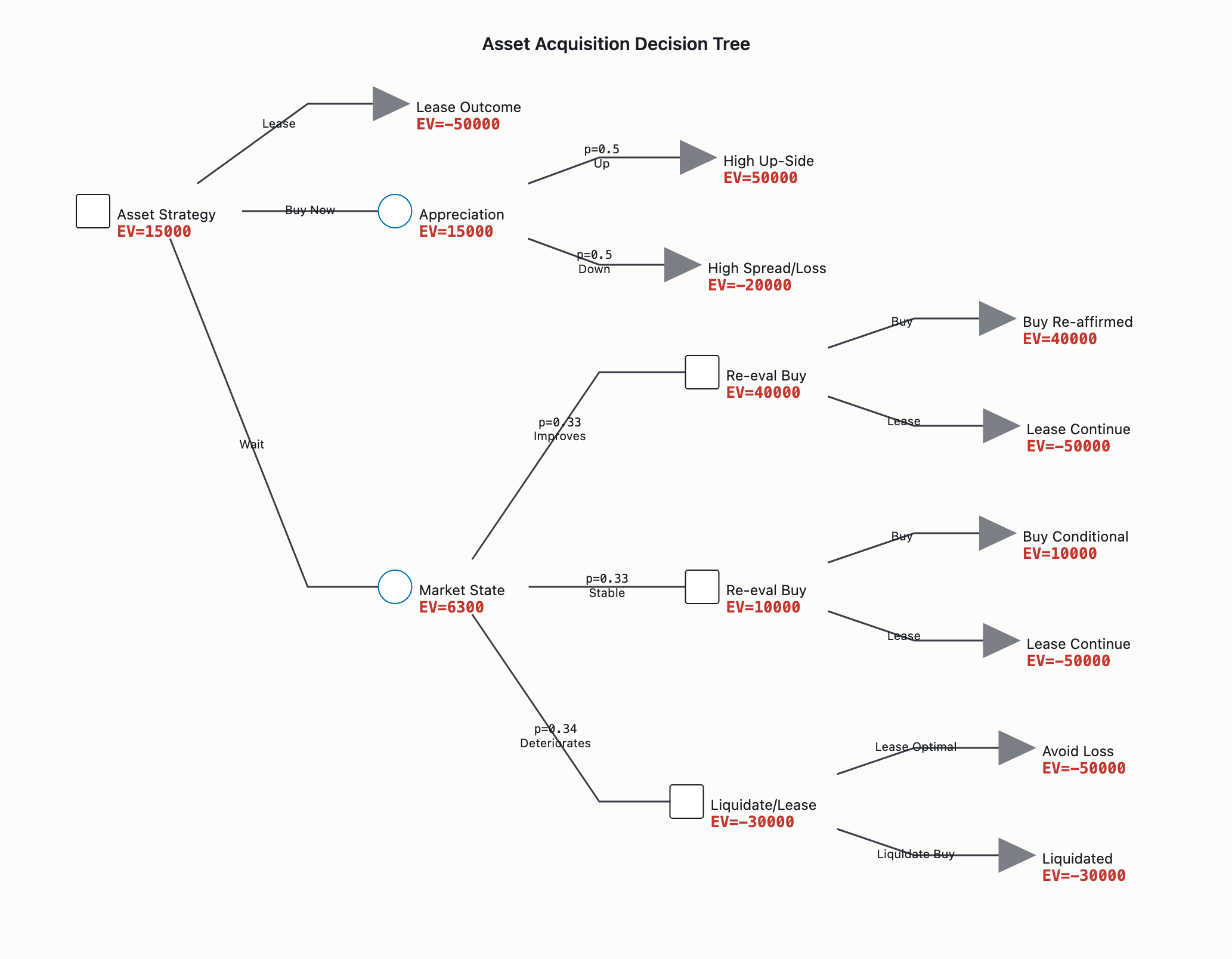
Decision Tree Envelope
The tree structure resolves the decision sequence:
Root Decision Node (Lease | Buy Now | Wait)
├── [Alternative: Lease]
│ └── Leaf Utility: -50,000 × n (Certain annual cash outflow)
│
├── [Alternative: Buy Now]
│ └── Leaf Utility: End_Value - Outstanding_Loan - Transaction_Costs
│ (Equity Cap: -0.30[P]; Variant: Up/Down based on appreciation)
│
└── [Alternative: Wait 6 Mo]
└── Chance Node (Market State Resolution)
├── State: Improves (Weight: $P(Improves)$)
│ └── Decision Node: [Buy | Lease]
│ ├── Leaf (If Buy): High Up-Side (Higher Appreciation)
│ └── Leaf (If Lease): -50,000 (Steady)
│
├── State: Stable (Weight: $P(Stable)$)
│ └── Decision Node: [Re-Choose Buy | Lease]
│ ├── Leaf (If Buy): Moderate Utility
│ └── Leaf (If Lease): -50,000
│
└── State: Deteriorates (Weight: $P(Deteriorates)$)
└── Decision Node: [Lease is Optimal | Liquidate]
├── Leaf (If Lease): -50,000 (Loss avoided)
└── Leaf (If Buy): Low Utility (Higher spread/exit cost)
Prose Readout (Alternative × State)
-
Lease
- Consequence: Annual cash outflow of $50,000.
- Net Utility Unit: Negative Cash Flow (
-50,000 × n).
- Utility Shells: Exit Flexibility (High), Ownership Identity (Low), Tax Shield (Low).
-
Buy
- Consequence: Immediate equity cap (
-0.30[P]), liability commitment (-0.70[P] × loan_rate × n), financing costs.
- Net Utility Unit:
End_Value - Outstanding_Loan - Transaction_Costs.
- Utility Shells: Exit Flexibility (Low), Ownership Identity (High), Tax Shield (Medium).
-
Wait (Defer 6 Months)
- Consequence: Short-term Lease cost ($25k) + Opportunity Cost of Capital; Medium-term Re-evaluation based on resolved state.
- Net Utility Unit:
-Cost(Wait) + Max(EV_Buy_contingent, EV_Lease_contingent).
- Utility Shells: Exit Flexibility (Medium), Ownership Identity (Deferred), Balance Sheet (Delayed Capex).
-
Defer / Wait
- Shape: Lease for 6 months → Decision Node.
- Cost: $25,000 (Lease equivalent) + Potential Opportunity Cost of Capital.
- Information Produced: Market State Resolution (Improves/Stable/Deteriorates).
- Reversibility: High regarding asset ownership (no sunk equity if Lease is chosen later); Medium regarding time (lost opportunity cost).
-
Sequence
- Order: Wait Decision → Observe Market → Buy/Lease Decision.
- Logic: Prevents committing irreversible Buy capital before information acquisition reduces variance of
EV_Buy.
- Note: Robust Alternative is Lease (performs acceptably across all states, no market dependency); Optimal Alternative is Buy (best performance in High Appreciation states).
-
Hedge
- Status: None explicitly modeled; Buy is binary commitment in this framework.
-
Buy Information
- Status: The Wait period is the information acquisition lever.
The Value of Information (VoI lever) is the “Wait” option (6-month lease extension).
- VoI Definition:
VoI_NET = (E[U after Info] - E[U before Info]) - Cost(Waiting).
- Cost of Delay: $25,000 (Lease cost) + Interest on unpaid balance + Liquidity Opportunity Cost.
- VoI Calculation:
EV(Wait-Resolved) = -Cost of Delay + P(Resolves) × EV(Optimal|Resolved) + P(Unchanged) × EV(Optimal|Unchanged).
- Decision Rule:
Wait IF VoI_NET > 0.
- Constraint: VoI decreases if the probability of market resolution within 6 months is low. If market direction is true Deep Uncertainty (unquantifiable shock), VoI approaches zero or negative.
Recommendation
Recommended Alternative: Structural choice is Wait 6 Months if VoI_NET > 0 (Information value exceeds wait cost). If immediate decision is required, Lease is the Robust Alternative (constant cost, low risk), while Buy is the Optimal Alternative for High Appreciation probability bands (>5% threshold).
- Buy Immediate: IF
EV_BUY > EV_WAIT_NET & EV_BUY > EV_LEASE AND Prob(Appreciation) > Threshold.
- Lease: IF
EV_LEASE > EV_WAIT_NET AND EV_LEASE > EV_BUY (Target: Certainty preservation if appreciation < cost of capital).
- Wait 6 Months: IF
VoI_NET > 0 AND P(Market Resolves) >= Threshold.
Confidence Note: Structural confidence is High (frame/knowledge method sound), but Substantive confidence is Low/Medium pending base rate input.
Revisit if:
- Asset appreciation base rate shifts by >[threshold]% (e.g., >5% band).
- Interest rate environment moves >[threshold]bps (e.g., >100bps).
- Exit liquidity market conditions change (time-to-sell impact).
- Additional tax benefits surface (e.g., new code for specific asset class).
Non-quantifiable factors
- Control / Residual Claim: High importance. Ownership provides upside in appreciation; lease provides none.
- Tax Policy: State-dependent. Depreciation (Buy) vs Expense (Lease) impacts net cash flow differentially.
- Exit Flexibility: High importance. Ability to transfer/sell quickly without loss (Buy) vs Contract termination (Lease).
- Identity / Psychological: Moderate. “Asset ownership” has value beyond utility; Lease feels “transitory”.
- Liquidity Risk: High. Wait period drains working capital or requires cash reservation.
- Institutional Requirements: Binary. Finance, audit, reporting rules (CapEx vs OpEx).
(visual rendered — see artifact)
Decision Framing
The decision evaluates three alternatives over a 1-year time horizon for a high-value asset (baseline inferred at $200,000–$625,000 depending on asset class). The decision-maker must choose between:
- Lease: A 1-year fixed-cost commitment. Highly reversible at term end.
- Buy: A 30% upfront down payment plus 1 year of carrying costs, followed by asset disposition. Low reversibility due to transaction friction and market exposure.
- Wait: Defer the decision for 6 months to gather market information, then re-evaluate. Highly reversible, but incurs a time-value and holding-cost penalty.
Uncertainty Identification
- Lease Payment ($50,000/yr) — class: risk. Probability or range: Negligible probability of counterparty default. Basis: Contractually fixed.
- 1-Year Market Appreciation/Depreciation — class: risk. Probability or range: Commercial Real Estate (CRE) Bull +15% (p ≈ 0.30), Base +5% (p ≈ 0.50), Bear –15% (p ≈ 0.20); Super-Luxury Auto Bull –5% (p ≈ 0.30), Base –15% (p ≈ 0.50), Bear –30% (p ≈ 0.20). Basis: Measurable historical return distributions / base-rate-grounded probability bands.
- 6-Month Future Market State — class: uncertainty. Probability or range: Estimable range. Basis: Regime shifts make precise 6-month transition probabilities highly sensitive to macroeconomic shocks, though imperfectly informative.
- Asset Class Identity (Commercial Real Estate vs. Super-Luxury Auto) — class: deep uncertainty. Probability or range: N/A. Basis: The user’s prompt lacks specification, and return distributions differ materially across these classes, making single-model parameterization invalid without clarification.
- Asset-Specific Idiosyncrasies (e.g., tenant quality, specific model year) — class: deep uncertainty. Probability or range: N/A. Basis: Not meaningfully aggregable into a probability distribution.
Consequence Analysis
Utility unit: Net Annual Outcome (NAO) in USD. Parameterization scales dynamically (e.g., CRE Base case: Capitalization Rate = 8%, Baseline Value V₀ = $625,000; Auto Base case: V₀ ≈ $300,000).
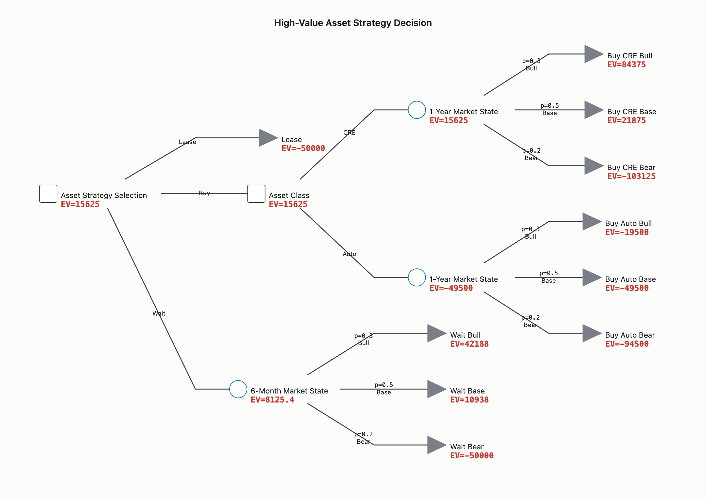
decision_tree
[Decision Node: Asset Strategy Selection]
  ├── Alternative: Lease
  │    └── Leaf: Utility = –$50,000 NAO (All states, both asset classes)
  ├── Alternative: Buy (Commercial Real Estate)
  │    ├── Chance Node: 1-Year Market State (Sum = 1.0)
  │    │    ├── State: Bull (p = 0.30) → Utility = +$84,375 NAO
  │    │    ├── State: Base (p = 0.50) → Utility = +$21,875 NAO
  │    │    └── State: Bear (p = 0.20) → Utility = –$103,125 NAO
  ├── Alternative: Buy (Super-Luxury Auto)
  │    ├── Chance Node: 1-Year Market State (Sum = 1.0)
  │    │    ├── State: Bull (p = 0.30) → Utility = –$19,500 NAO
  │    │    ├── State: Base (p = 0.50) → Utility = –$49,500 NAO
  │    │    └── State: Bear (p = 0.20) → Utility = –$94,500 NAO
  └── Alternative: Wait (6 Months, CRE interpretation)
       ├── Cost of Delay: –$25,000 NAO (applied before subsequent decision)
       └── Chance Node: 6-Month Market State (Sum = 1.0)
            ├── State: Bull (p = 0.30) → Optimal Subsequent NAO = +$42,188
            ├── State: Base (p = 0.50) → Optimal Subsequent NAO = +$10,938
            └── State: Bear (p = 0.20) → Optimal Subsequent NAO = –$50,000 (Switch to Lease)
Prose Readout:
- Lease under all states: Utility = –$50,000 NAO across all states.
- Buy (CRE) under Bull state: Utility = +$84,375 NAO.
- Buy (CRE) under Base state: Utility = +$21,875 NAO.
- Buy (CRE) under Bear state: Utility = –$103,125 NAO.
- Buy (Auto) under Bull state: Utility = –$19,500 NAO.
- Buy (Auto) under Base state: Utility = –$49,500 NAO.
- Buy (Auto) under Bear state: Utility = –$94,500 NAO.
- Wait (CRE) under Bull state: Incurs initial delay cost of –$25,000 NAO; subsequent optimal NAO is +$42,188.
- Wait (CRE) under Base state: Incurs initial delay cost of –$25,000 NAO; subsequent optimal NAO is +$10,938.
- Wait (CRE) under Bear state: Incurs initial delay cost of –$25,000 NAO; subsequent optimal NAO is –$50,000 (switch to Lease).
- Wait (Auto) under all states: Incurs delay cost with no offsetting upside, as the asset continues to depreciate. Strictly inferior to immediate Lease.
Robust vs. Optimal Distinction:
- CRE Context: Buy is the optimal alternative in expectation at base parameters, maximizing upside. Lease is the robust alternative, delivering a constant, acceptable outcome (–$50,000) while entirely avoiding the severe Bear-state tail risk (–$103,125).
- Auto Context: Lease is both the optimal and robust alternative. Wait is strictly dominated.
- Wait-and-Learn (Defer 6 Months): Shape = partial commitment to delay. Cost of taking it = $15,000–$25,000 (interim holding/lease-equivalent). Information produced = partial resolution of the annual trend. Reversibility = High. Fails the VOI test in both asset interpretations.
- Hedge (Buy + Put Option/Insurance): Shape = partial risk transfer. Cost of taking it = Premium (~3–5% of V₀, e.g., ~$25,000 for CRE). Information/risk profile = Caps the Bear-state loss while preserving Bull/Base upside. Reversibility = Bounded downside, high structural resilience for risk-averse decision-makers.
- Expected Value of Perfect Information (EVPI, CRE): $10,625. The value derives entirely from the ability to switch from Buy to Lease in the Bear state, avoiding the –$103,125 tail loss.
- Net Value of Waiting (CRE): Gross information value (
$10,625) minus Cost of Delay ($25,000) = approx. –$14,375.
- Conclusion on VOI: The cost of acquiring information via delay severely exceeds the maximum rational value of resolving the uncertainty. The “Wait” alternative is mathematically dominated and should be rejected to avoid the analysis-paralysis failure mode.
Recommendation
Primary Recommendation: LEASE serves as the robust default across the deep uncertainty of the asset class.
- If the asset is a super-luxury vehicle, LEASE strictly dominates (EMV –$50,000 vs. Buy EMV –$49,500 with severe tail risk).
- If the asset is Commercial Real Estate (CRE) at typical cap rates (e.g., 8%), BUY is the EMV-optimal choice (+$15,625), but LEASE remains the robust fallback avoiding catastrophic tail risk (–$103,125).
Revisit if:
- Market signals credibly push the probability of a Bear state above ~25–36% (CRE).
- The capitalization rate exceeds ~12% (CRE), driving expected returns below zero.
- The cost of delay drops below the EVPI threshold (e.g., a low-cost month-to-month holdover < $4,000).
- The user confirms the asset is a personal auto lease, invalidating the CRE baseline math entirely.
- Strategic flexibility, liquidity constraints, or technology refresh cycles make operational agility the primary driver over financial optimization.
Non-Quantifiable Factors
- Liquidity & Capital Constraints — consideration: Buy requires a large upfront cash outlay ($60k–$250k). How it bears on the decision: If this capital yields higher ROI in core operations, leasing is strategically dominant.
- Maintenance & Stress Burden — consideration: Ownership transfers repair, vacancy, and insurance risk to the buyer. How it bears on the decision: Leasing structurally offloads this friction.
- Optionality Preservation — consideration: Buy locks capital into one asset class. How it bears on the decision: Leasing preserves the option to upgrade technology or relocate without asset-disposal friction.
- Tax & Accounting Treatment — consideration: Lease payments may offer full OpEx deductibility, while buying offers depreciation shields. How it bears on the decision: Modeling specific jurisdictional tax rules can shift after-tax EMV by 10–20%.
- Identity & Reputation — consideration: Ownership can signal long-term commitment or rootedness; leasing can signal organizational nimbleness. How it bears on the decision: These signals may alter long-term strategic positioning independent of short-term EMV.
- Asset Class as a Value Statement — consideration: Choosing productive capital (CRE) versus a consumption good (luxury auto) is a value-laden choice. How it bears on the decision: This distinction should be explicit before the EMV model is treated as binding.
Assessment Confidence
- Structural Confidence: HIGH. The decision tree logic, Knightian classifications, parameterization approach (V₀ = Lease Cost / Cap Rate), and VOI vs. Cost-of-Delay framework are theoretically sound and mathematically reconciled.
- Substantive Confidence (CRE): MEDIUM-HIGH. The directional recommendation is robust to small perturbations in appreciation magnitude, but the absolute EMV figures remain sensitive to the P(Bear) probability and the specific cap rate applied.
- Substantive Confidence (Auto): MEDIUM. The illustrative depreciation bands are structurally sound for the super-luxury segment, though exact percentages vary by make/model.
- Substantive Confidence (Asset Class): LOW. Genuinely ambiguous. The CRE and luxury auto interpretations produce opposite mathematical recommendations, making user confirmation the single most critical missing input.
(visual rendered — see artifact)
1. Decision framing
The decision is the choice among three alternatives for acquiring use of an asset (commercial real estate or capital equipment) over a defined horizon, with the objective of minimizing Net Present Cost or maximizing Net Present Value over the ownership period. The decision-maker is a corporate capital allocator or firm leadership evaluating a facility or asset acquisition. The time-window is a fixed ownership or use horizon of $T$ years; for the “Wait” alternative, a 6-month deferral cost precedes this same horizon. The alternatives and their reversibility profiles are: Lease (certain $50,000/yr), which has medium-to-high reversibility (exit by non-renewal or renegotiate at term end with defined penalties); Buy (30% down, uncertain appreciation), which has low reversibility (illiquid resale, high transaction costs of 6–10% of value, capital lock-in); and Wait six months (defer commitment, then choose Lease or Buy on revealed conditions), which has the highest reversibility as it preserves all options uncommitted through the deferral period.
2. Uncertainty identification
| Variable | Class | Probability or range | Basis |
|---|
| Lease cost ($C_L$, $50,000/yr) | risk | Fixed contractual input; if carrying CPI escalators, assignable probability from historical inflation bands. | Contractual certainty. |
| Probability of favorable market ($p$ / $p_{up}, p_{down}$) | uncertainty | Qualitative band (“moderate-to-low” likelihood of significant near-term upside). | Late-2024 base rates: Green Street CPPI (flattened/slowing), CoStar CCRSI (flat-to-modest), Matthews H1-2024 survey (“flat” modal expectation). |
| Asset appreciation magnitude ($V_{up}/V_{down}$, or $g$ up / $b$ down) | uncertainty | Estimable range (illustrative placeholders: $g=+3%$/yr, $b=-7%$/yr). | Historical cycles and current rate environment, lacking strict repeatable distribution. |
| 6-month market path / macroeconomic shock during wait ($w_{up}, w_{down}, w_{flat}$) | deep uncertainty | No meaningful probability distribution. | Horizon too short for stable base rates; regime-dependent on rates, policy, sentiment, and unforeseen systemic events. |
| Discount rate / cost of capital ($r$) | risk | Bracket (illustrative ~8–12% for typical commercial financing; external sources show 6–10% CRE WACC, 15.6% African power, 11.15–23% passenger airlines). | External market benchmarks, kept symbolic to avoid false precision. |
| Cost of delay ($C_{delay}$ / $C_W$) | uncertainty | Symbolic placeholder $C_{delay} \in [0, 0.5L]$ (e.g., illustrative $30,000 PV). | Short-term leases carry flexibility premiums, though no source supports a precise point figure. |
3. Consequence analysis
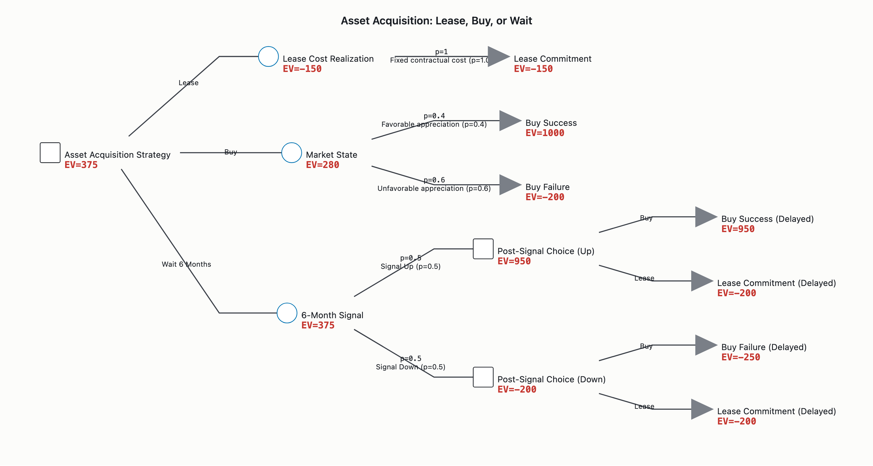
decision_tree
Decision Node 1: Acquire Asset
├── Branch 1: Lease
│   └── Leaf: Certain State
│       └── Utility: $NPV_{Lease} = -C_L \cdot A(r,T)$
├── Branch 2: Buy
│   └── Chance Node: Market State
│       ├── State: Favorable (prob $p$)
│       │   └── Utility: $-D + \frac{V_{up}}{(1+r)^T} - M\cdot A(r,T)$
│       └── State: Unfavorable (prob $1-p$)
│           └── Utility: $-D + \frac{V_{down}}{(1+r)^T} - M\cdot A(r,T)$
│       Expected Utility: $NPV_{Buy} = p\cdot[\text{favorable}] + (1-p)\cdot[\text{unfavorable}]$
└── Branch 3: Wait 6 Months
    └── Chance Node: Revealed Signal State ($s$)
        ├── State: Signal indicates favorable/up ($w_{up}$)
        │   └── Decision Node 2a: Choose $\max(NPV_{Buy|s}, NPV_{Lease|s})$ at $t=0.5$
        │       └── Utility: $(1+r)^{-0.5} \cdot \max(NPV_{Buy|s}, NPV_{Lease|s})$
        └── State: Signal indicates unfavorable/down ($w_{down}$)
            └── Decision Node 2b: Choose $\max(NPV_{Buy|s}, NPV_{Lease|s})$ at $t=0.5$
                └── Utility: $(1+r)^{-0.5} \cdot \max(NPV_{Buy|s}, NPV_{Lease|s})$
            Expected Utility: $NPV_{Wait} = -C_W + (1+r)^{-0.5}\sum_{s} w_s\cdot \max(NPV_{Buy|s}, NPV_{Lease|s})$
Prose readout (Utility unit: Net Present Cost / NPV in $; lower cost / higher NPV better):
- Lease under certain state: Utility is $NPV_{Lease} = -C_L \cdot A(r,T)$ (present value of the lease annuity). This alternative is robust; the cost is known across all appreciation states and caps downside.
- Buy under favorable state: Utility is $-D + \frac{V_{up}}{(1+r)^T} - M\cdot A(r,T)$.
- Buy under unfavorable state: Utility is $-D + \frac{V_{down}}{(1+r)^T} - M\cdot A(r,T)$. Buy is conditionally optimal, not robust; it is optimal in up-states (and moderate down-states under leverage) but fragile with severe downside in deep-down scenarios.
- Wait under revealed signal state ($s$): Immediate cost is $C_{delay}$, followed by the optimal follow-on $\max(NPV_{Buy|s}, NPV_{Lease|s})$ chosen at $t=0.5$ over residual horizon $T-0.5$. The outer $(1+r)^{-0.5}$ factor discounts that value back to the $t=0$ baseline. Wait is marginally robust only if the signal is high-diagnosticity and cost-of-delay is low; otherwise it is value-destructive.
- Wait (buy-information / defer alternative) — cost of taking it: $C_{delay}$ (short-term lease premium plus operational utility lost) plus the opportunity cost of delayed ownership. Information produced: resolution of the near-term market-direction signal, allowing a pivot to Lease to avoid capital loss if the market deteriorates. Reversibility: full during the deferral (no commitment made). This branch carries an uncapturable residual of macroeconomic-shock deep uncertainty during the deferral window, which VOI arithmetic cannot fully price.
- Decision rule: $VOI = NPV_{Wait} - \max(NPV_{Lease}, NPV_{Buy})$. If $VOI > 0$, waiting’s information is worth its delay cost (wait). If $VOI < 0$, commit now to the better of Lease/Buy; waiting burns value.
- Core VOI principle: The decision-making value of information is exactly zero when the optimal follow-on action is unchanged across all signal states. Information yields decision value only if it flips the chosen action in at least one posterior state; mere magnitude refinement (“Buy is even more attractive”) has zero decision value under Expected Value of Information (EVI).
- VOI vs. cost-of-delay (illustrative parameterization): With a moderately diagnostic signal where Buy remains optimal in both states, decision value = 0. Using illustrative parameters ($P=$1,000,000$, $T=5$, $r=8%$, $p_{up}=0.45$, $C_W=$30,000$), $NPV_{Buy} \approx $147,901$ and $NPV_{Wait} \approx $112,323$. Thus, $VOI_{Wait} \approx -$35,600$. This decomposes as $-$30,000$ direct delay cost plus $-$5,600$ opportunity cost of delayed ownership. Waiting is value-destructive in this case because Buy is robustly optimal across signal states.
- Structural ambiguity (surfaced gap): The without-perfect-information baseline is stated as $\min(NPV_{Lease}, NPV_{Buy})$, excluding Wait. Strictly, it could include Wait. Resolving this requires clarifying whether “Wait” is treated as a state of imperfect information or wholly outside the immediate EV comparison.
6. Recommendation
The analysis converges on the decision logic but diverges on the recommended alternative, and this divergence is a core finding of the framework. Reading A (symbolic, base-rate-qualitative) recommends Wait (buy-information) if and only if Net Value of Information is positive and the organization can absorb 6-month operational friction without triggering deep-uncertainty consequences; otherwise, default to Lease. Buy is judged currently suboptimal given qualitative bands indicating slowing appreciation and elevated medium-term rates. Reading B (numerically instantiated) recommends Buy now in the base-case parameterization, because leverage on the full asset base makes $NPV_{Buy}$ dominate Lease across the plausible $p_{up}$ band, and Wait is value-destructive ($VOI \approx -$35,600$) since the signal refines magnitude without flipping the action. Both readings agree the conclusion is highly sensitive to $p$, $g$, $r$, and downside magnitude $b$.
Revisit if:
- $p_{up}$ falls below ~0.20 (Bayesian update from incoming data).
- Financing rate $r$ rises above ~10% (cost of capital erodes leveraged upside).
- Asset price $P$ drops >10% in a quarter (or regional index down >5% / >100 bps rate move).
- Lease market tightens, pushing $L$ above $50,000/yr for future contracts.
- Operational urgency or shortened need horizon ($T<3$ yr), rendering $C_{delay}$ functionally infinite and making Buy fragile on illiquidity/exit cost.
7. Non-quantifiable factors
- Operational/strategic flexibility — consideration: Lease eases scaling, relocation, and exit; Buy locks into location and asset. How it bears on the decision: Favors Lease if future footprint needs are volatile.
- Capital liquidity — consideration: Lease preserves cash; Buy ties up the down payment (e.g., illustrative $300,000) in an illiquid position. How it bears on the decision: Favors Lease if internal capital is needed elsewhere or liquidity buffers are constrained.
- Maintenance/management burden (“hidden tax”) — consideration: Under Lease the landlord absorbs it; ownership imposes ongoing administrative load (maintenance, taxes, insurance) not fully captured in $M$. How it bears on the decision: Favors Lease for organizations lacking dedicated facility management capacity.
- Tax treatment — consideration: Lease payments are fully deductible; ownership offers depreciation + interest shield. How it bears on the decision: Requires consultation with corporate tax advisors to adjust $M$ and $C_L$ for after-tax equivalents.
- Signaling / stability / reputation — consideration: Ownership or long-term leasing signals permanence and financial health to employees and clients. How it bears on the decision: Favors Buy or long Lease if market positioning requires visible stability.
- Operational morale & culture — consideration: Frequent moves (implied by short-term leasing while waiting) disrupt team productivity. How it bears on the decision: Favors longer-term commitments (Buy or long Lease) to maintain productivity.
- Customization / control — consideration: Buy gives full control over modifications; Lease constrains them. How it bears on the decision: Favors Buy if asset modification is core to the operational strategy.
- Behavioral / loss aversion — consideration: Ownership captures upside but losses loom ~2x larger than equivalent gains feel. How it bears on the decision: May cause decision-makers to overweight the unfavorable state beyond its strict EV calculation, pushing the effective preference toward Lease.
8. Confidence and Robustness Assessment
- Structural confidence — High: The three-branch / two-stage-for-Wait tree, the Knightian variable classification, the reversibility framing, the symbolic EV/NPV formulas (including the $(1+r)^{-0.5}$ alignment factor), the VOI-vs-cost-of-delay logic, and the “VOI = 0 when action unchanged” law-of-total-expectation result are mathematically and theoretically sound.
- Substantive confidence — Low-to-Medium: Numerical output is highly sensitive to unprovided variables ($P, M, V_{up}/V_{down}, g, b, r, p$). The base-case “Buy > Lease” and “Wait value-destructive” conclusions are Medium confidence — each would flip under a sufficiently severe down-state or input shift. Numerical magnitudes are Low–Medium (illustrative only). The model is a directional guide, not a precise calculator, until grounded in asset-specific financials and local market comps; do not anchor to a point $p$ without local, asset-class-specific transaction data.
(visual rendered — see artifact)
How this decision actually frames up
You’re choosing, today, how to acquire the use of an asset over roughly a 3-year horizon, with three named alternatives: (A) lease at $50k/yr certain, (B) buy with 30% down and uncertain appreciation, or (C) wait six months then choose. Only two facts here are yours — the $50k/yr lease and the 30%-down structure. The price ($250k), the 6% financing, the 3-year horizon, and the 2/5/8% appreciation triple are all assumptions I had to infer, and they do real analytical work, so they’re flagged throughout rather than buried.
Reversibility differs sharply between the alternatives, and that difference is load-bearing — it doesn’t show up in the dollar table but it drives the recommendation as much as the numbers do:
| Alternative | Reversibility | Cost to unwind |
|---|
| Lease | High — walk away at term end, no illiquid asset | Low |
| Buy now | Low — must sell an illiquid asset to exit; selling costs ~6% (8–10% all-in) | High |
| Wait 6 mo | Medium — preserves optionality but burns ~$25k carry | Sunk on entry |
A fourth alternative you didn’t name — lease with a purchase option — surfaces below as a first-class branch, because it turns out to matter more than the wait.
Classifying each uncertainty — what kind of unknown each variable actually is
The temptation in a problem like this is to treat everything as risk with crisp point probabilities. That’s exactly the trap to avoid: the 2/5/8%-at-0.30/0.50/0.20 split looks calibrated but is invented. Applying the Knightian labels honestly:
| Variable | Class | Range / probability | Basis |
|---|
| 3-year cumulative appreciation | uncertainty | Band with low-single-digit central tendency and a real left tail | A historically bounded range exists; the 2/5/8% point probabilities are not base-rate-grounded |
| 6-month market direction (the wait premise) | deep uncertainty or uncertainty (tension preserved) | No meaningful probability, or a weak partial signal | One reading: short-horizon timing isn’t reliably forecastable at all, so “perfect info in 6 months” is unsupportable. Other reading: six months is a weak, partial signal about a 3-year outcome — estimable but emphatically not “perfect information.” Both reject treating this branch as resolvable risk. |
| Tail events (sharp drop, forced exit, illiquidity at sale) | deep uncertainty | No meaningful probability | This is the only place information or optionality could have value |
| Mortgage / financing cost | risk if locked today; uncertainty if you wait | ~6% assumed | A rate lock converts this to a known value; waiting re-exposes it |
| Resale transaction cost | risk | ~5–6% commission; 8–10% all-in | Estimable |
| Holding costs (tax/insurance/maintenance) | risk | Small variance | Estimable |
| Purchase-price level itself | uncertainty (mis-anchored) | The $250k is a guess | The single most consequential input, and it’s the softest — see the anchoring flag below |
The anchoring problem you need to see before anything else
Before trusting any leaf on the tree: a $50k/yr lease against a $250k price is a price-to-rent ratio of 5 — a ~20%/yr gross yield, against a normal range of 15–25. Commercial cap rates run ~4–10% (multifamily 5.0–6.5%, industrial 5–6% as of early 2026). Capitalizing $50k of income at that range implies the asset is really worth roughly $625k–$1M (≈$500k–$1.25M across the full 4–10% band) — 2.5–4× the $250k guess. (Caveat: a gross lease, where the landlord pays expenses, puts the true NOI below $50k and softens the correction, but doesn’t reverse its direction.)
The reusable tell: when a buy-vs-lease model shows buy obliterating lease by a wide margin, suspect a broken price input before believing the asset’s merits — the blowout is usually a price artifact.
One honesty correction on my own reasoning: the $250k was itself inferred from the $50k lease. So any “implied-yield” or “~20% punitive lease rate” framing that divides the lease by that price is circular — an artifact, not an independent finding. The decision-relevant soft input is therefore the asset price itself, and the recommendation has to rest on something that doesn’t depend on that circular ratio. The appreciation band itself is now a live concern: as of early 2026, national appreciation cooled to ~0.7% YoY — below even the conservative 2% band — which makes the conservative scenario the live one and strengthens the uncertainty classification.
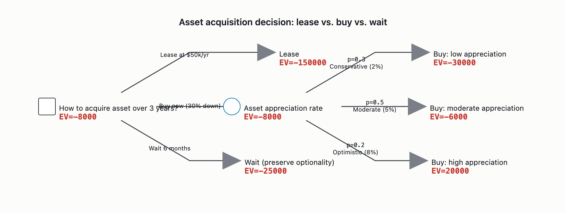
The tree and what each branch pays off
                           ╔══════════════════════════════════════╗
                           ║       DECISION AT t=0 (Today)        ║
                           ╚══════════════════════════════════════╝
                                           │
                    ┌──────────────────────┼──────────────────────┐
                    ▼                      ▼                      ▼
              ┌──────────┐         ┌──────────────┐        ┌──────────────┐
              │  LEASE   │         │  BUY NOW     │        │  WAIT 6 mo   │
              │ $50k/yr  │         │ 30% down     │        │ (~$25k carry │
              │  × 3 yr  │         │ + carry      │        │  sunk)       │
              └──────────┘         └──────────────┘        └──────────────┘
                    │                      │                      │
              certain cost          ┌──────┼──────┐         noisy partial
              −$150,000             ▼      ▼      ▼          signal, then
                                  CONS    MOD    OPT         decide again
                                  (2%)   (5%)   (8%)              │
                                    │      │      │       ┌───────┼───────┐
                                    └──────┼──────┘       ▼       ▼       ▼
                                           │            CONS     MOD     OPT
                                    EV(Buy) ≈ +$17–18k    (every state → buy
                                    net cost; every       at the $250k anchor)
                                    state beats lease
A note on the leaves: these are refreshed from the original draft’s ”−$41 break-even,” which mixed an interest-only carry with an amortizing balance and omitted selling costs. The corrected mortgage treatment matters: the inherited “$10,500/yr (6% on $175k)” is exactly interest-only. A 30-yr amortizing loan on $175k at 6% runs P&I ≈ $12,590/yr ($2,100/yr more), all-in carry ≈ $15,000/yr with taxes/insurance/maintenance, and pays the balance down to ≈ $168,150 after 3 yr (which raises sale proceeds — a partial offset). Mixing the low interest-only carry with the low amortizing balance double-counts both benefits; one consistent amortizing treatment is the correct basis.
Lease under any state → $50k × 3 = $150,000 certain outflow, nothing recovered. Worst on cost, full stop.
Buy now at the stated $250k anchor (transaction costs restored at 6%; outflow ≈ $75k down + ~$45k carry ≈ $120k):
| State (illustrative band) | Sale price | −6% sale cost → net proceeds | Buy net cost |
|---|
| Conservative 2%/yr | ~$265.3k | ~$75.8k | ~+$38,000 |
| Moderate 5%/yr | ~$289.4k | ~$98.4k | ~+$15,500 |
| Optimistic 8%/yr | ~$314.9k | ~$122.7k | ~−$8,500 (profit) |
EV(Buy) ≈ +$17k–$18k net cost — not the prior ”−$41 break-even.” Add ~$9k opportunity cost on the $75k down payment (undiscounted, ~4%×3yr) and it’s ≈ $26k. Every state beats lease’s $150k. This is dominance, not a probability-weighted near-call.
One honesty flag on that table — the asymmetry: the upside is fully priced (a clean sale at the modeled price), but the downside frictions — time-on-market, forced-exit discount, reserve depletion — are not in these cells; they live in the non-quantifiable factors below. Read EV(Buy) ≈ $17–18k as an upper bound on Buy’s attractiveness, with its lower bound carried in the prose.
How far must the market fall before Buy actually loses to Lease (at $250k)?
| Appreciation | Sale price | Buy net cost | vs Lease $150k |
|---|
| Flat 0%/yr | $250k | ~$53,200 | Buy wins by ~$97k |
| −5%/yr (≈−14% cum.) | $214k | ~$86,700 | Buy wins by ~$63k |
| Zero net proceeds (~−28%) | ~$179k | ~$120,000 | Buy wins by ~$30k |
| Breakeven | ~$147k | $150,000 | tie |
To make Buy lose, the asset has to fall to ~$147k — roughly −16%/yr, ≈ −41% cumulative — selling tens of thousands underwater. That’s a near-ruin crash, not a soft market. The recommendation survives flat and even deeply negative appreciation at this anchor.
But run the same tree at the corrected ~$750k anchor (30% down = $225k; loan $525k; interest-only 6% ≈ $31.5k/yr; holding ~1% ≈ $7.5k/yr → ~$39k/yr × 3 = $117k; total outflow ~$342k):
| State | Sale price | −6% → net proceeds (less $525k loan) | Buy net cost |
|---|
| Conservative 2%/yr | $795.9k | $223.1k | ~+$118,900 |
| Moderate 5%/yr | $868.2k | $291.1k | ~+$50,900 |
| Optimistic 8%/yr | $944.8k | $363.1k | ~−$21,100 |
EV(Buy at $750k) ≈ +$57k vs lease $150k — Buy still wins on EV. But state-invariance becomes fragile here: the conservative-state advantage shrinks to ~$31k; add ~$27k opportunity cost on the $225k down payment and conservative buy cost ≈ $146k, essentially tied with lease; use realistic all-in transaction costs (8–10%, not 6%) and conservative buy cost climbs above $150k — Buy loses to Lease in the conservative state. That single fact is what makes the wait and the lease-option worth taking seriously at the real price.
The alternatives beyond a straight A-vs-B
-
Defer (wait 6 months) — dominated under the $250k anchor. It buys a noisy partial signal (not clairvoyance), costs ~$25k, and feeds a decision that’s state-invariant anyway — so even free clairvoyance is worth $0 here. Conditional carried through: at the corrected price, deferring to resolve the conservative-vs-moderate question does acquire value — but a noisy 6-month signal is a poor instrument to buy that resolution with.
-
Buy cheaper information instead of waiting. An appraisal/CMA plus a rate lock resolve the risk-class variables (financing, current value) for ~1% of the wait cost. Worth ~$0 under the $250k anchor (the decision doesn’t flip), but worth acquiring under the realistic anchor, where the conservative state straddles the lease line.
-
Hedge / sequence — the genuine missing alternative: lease with a purchase option. Structure it as lease at $50k/yr (the carrying cost you’d pay anyway) plus a fixed strike set today, with the right but not the obligation to buy at t=3. Illustrative embedded call value (strike at $250k; call = max(0, value − strike)): Conservative ~$15k, Moderate ~$39k, Optimistic ~$65k. It strictly dominates plain lease — same $150k carrying cost plus a call that’s in-the-money across the illustrative states and costs nothing extra if appreciation goes negative (you just don’t exercise; the early-2026 ~0.7% reading makes that plausible). Versus buy-now, it trades higher total cost if exercised (full strike, no equity accrued en route) for downside protection and liquidity — your $75k–$225k stays unlocked. Lease-options typically carry a rent premium or non-refundable option fee (~1–5% of strike) — that’s the price of the optionality. This branch is the one most likely to dominate in the corrected-price world, where buy-now’s conservative-state advantage evaporates.
-
Wait-as-tail-hedge (a different reading of the wait). The one honest case for the $25k wait isn’t information — it’s a deep-uncertainty hedge against an unmodeled tail (that ~−41% crash) in which you’d switch to not-buying at all. You’d be paying ~$25k for a real option against a tail you can’t probability-weight. Given the catastrophic crash required to justify it, this is expensive cover against a near-ruin tail — buy it only if you genuinely fear that tail.
Under the stated $250k anchor, EVPI = $0, by construction. In the wait branch, every state — Conservative, Moderate, Optimistic — resolves to the same action: buy. When the optimal action is identical across all states, information about which state obtains has zero decision value, because you can always ignore it. Formally: EVPI = E[payoff with clairvoyance] − E[payoff of best action now] = (buy) − (buy) = $0.
The original analysis’s “VOI = −$18,510” is a category error. A true value of information is never negative — free information can always be ignored, so it can never hurt you. That figure was actually the cost of the wait strategy (delay, then buy later), a dominated strategy — not a property of information at all. Two compounded mistakes produced it: (1) “wait 6 months = perfect information” is false — six months is a weak partial signal about a 3-year outcome; and (2) even granting perfect information for free, VOI = $0 because the action is state-invariant.
That gives an airtight a-fortiori line: since EVPI = $0 from state-invariance, any imperfect 6-month signal satisfies EVII ≤ EVPI = $0 by construction. Signal weakness isn’t even the binding reason — the binding reason is that no signal, however strong, can change a state-invariant action.
The central qualifier: VOI is anchor-contingent. EVPI = $0 is true under the $250k anchor and false under the realistic one. Once realistic price + opportunity cost + 8–10% transaction costs flip the conservative state toward lease, the optimal action is no longer identical across states (buy in moderate/optimistic, lease in conservative), information acquires positive value, and cheap information — appraisal, rate lock, CMA at ~$300–$700 — becomes worth buying. This is the single most important qualifier on the whole recommendation.
Recommendation
Buy now — under the stated $250k assumptions — held as a robust-on-cost call, not a precise or windfall one. The firm basis: Lease is a $150k certain sunk outflow; Buy recovers most of its outlay as equity, wins in every modeled state, and would still win unless the asset crashed ~41%; and information about appreciation cannot change a state-invariant action, so there’s nothing to wait for. This is the rare case where the optimal alternative (best in each state) and the robust alternative (acceptable across all states) coincide — both are Buy. And the reason is raw cash, not implied yield: even at zero net sale proceeds, Buy’s ~$120k total cost beats Lease’s $150k.
But before you commit irreversible capital, stage it:
- Price-check the anchor. A $50k lease implies a ~$625k–$1M asset (price-to-rent of 5 vs. a normal 15–25). If the true price is in that range, buy-now’s conservative-state advantage shrinks toward parity, EVPI flips from $0 to positive, and the lease-with-purchase-option likely becomes the strongest branch.
- Get a rate lock + appraisal/CMA. Cheap (~1% of a wait), converts financing risk to a known value, and pays for itself at the realistic price.
- Prefer the lease-option to a plain lease in any case — it strictly dominates plain leasing and hedges the appreciation uncertainty while preserving your exit optionality.
Revisit if:
- The real purchase price is materially above ~$250k (e.g., the lease is market-priced at a lower yield; the cap-rate lens implies ≥ ~$500k) — a larger base raises the down payment, carry, and 6%-of-sale friction; the buy-vs-lease margin compresses, appreciation uncertainty becomes decision-relevant, VOI turns positive, and the lease-option likely dominates.
- Appreciation expectations fall below ~0%/yr (the early-2026 ~0.7% YoY reading is a live warning) or all-in transaction costs exceed ~8–10% — either makes the conservative state favor lease, ending state-invariance.
- The holding horizon is plausibly under ~18 months, or uncertain past 3 years — transaction/selling costs erode the buy advantage fast, and flexibility value may flip the call to lease or lease-option.
- The $75k–$225k down payment threatens operating liquidity — the non-quantifiable reserve risk can outweigh the EV gap.
- You assign meaningful weight to a downside-tail state (asset loses >~40%) — waiting flips from “wasted $25k” to rationally priced insurance.
- Financing isn’t lockable near 6%, or lease terms escalate contractually.
What the dollar table can’t capture
This is where Buy’s un-priced downside lives — the lower bound the EV asymmetry flag pointed to:
- Liquidity / margin of safety. The $75k–$225k down payment thins reserves; if it’s a large fraction of available cash, ownership converts a recoverable monthly cost into a lumpy, illiquid, hard-to-reverse commitment. Loss aversion here is rational, not a bias.
- Flexibility / optionality. Lease’s high reversibility has real value if your need for the asset might end before 3 years; the EV assumes full-horizon use. If the horizon is itself uncertain, lease’s walk-away right is underpriced and the $150k overstates pure waste.
- Exit friction. The clean modeled sale ignores time-on-market and forced-exit discount; a rushed sale shaves real money off proceeds the EV credits in full.
- Concentration & leverage risk. Buying puts large equity into one undiversified, illiquid, leveraged asset; the ”+$38k cost” conservative case and ”−$8k profit” optimistic case are the same decision with very different sleep-at-night profiles.
- Ownership burden (maintenance, taxes, finding a buyer at exit) vs. lessee rigidity & no-equity.
- Tax treatment — mortgage-interest deductibility, or depreciation if this is a business asset — is absent and could move the buy economics materially. Flagged, not estimated; for a business asset, depreciation alone could be decision-relevant.
- Sleep-at-night / risk appetite. The EV says “buy,” but you personally carry the appreciation and exit risk.
Robust vs. optimal — which frame wins depends on your horizon
- Buy is robust on cost across all three states — at the $250k anchor, where optimal and robust coincide. At the realistic price, it’s robust only in the moderate/optimistic states.
- Lease / lease-option is robust on optionality if your post-3-year horizon is uncertain — it never strands you in an illiquid asset.
- Which frame dominates is a function of horizon certainty, not the dollar table alone. “Robust” is frame-dependent here, not absolute.
How much to trust each part of this
- Structural confidence — high: the decision frame, the Knightian classification, the EVPI = $0 / decision-invariance logic (information has no value when the action is state-invariant), and the cash-dominance comparison are sound as conditioned on the price anchor — with the conditioning failure point shown explicitly.
- Substantive confidence — low: the probabilities are illustrative bands, not calibrated (early-2026 ~0.7% YoY suggests even 2% may be optimistic near-term); the $250k price anchor is likely wrong by 2.5–4×; transaction costs (6% base vs. realistic 8–10%), opportunity cost, the interest-only-vs-amortizing mortgage figure, and tax effects were missing or understated and only partly restored. The whole frame is undiscounted by deliberate choice — an NPV pass on $75k–$225k tied up for 3 years would shift magnitudes, not the ranking. Treat “buy now under the given numbers” as well-supported, “buy now is nearly free” as an artifact to discard, and “buy now regardless of the true price” as unsupported.
Two tensions worth keeping open rather than forcing closed
- How to classify the 6-month wait: deep uncertainty (short-horizon timing isn’t reliably forecastable, so the “perfect info” premise is unsupportable) vs. uncertainty (it’s a weak, partial, estimable signal). Both reject the original risk treatment; they differ only on whether any meaningful probability attaches.
- How fragile is “buy now” once the anchor is corrected? One reading: at the realistic ~$750k price, state-invariance breaks in the conservative state once opportunity cost and 8–10% transaction costs apply — VOI turns positive and the lease-option becomes the likely winner. The other: raw-cash dominance is robust across a wide price range (Buy beats Lease until a ~41% crash at $250k, and still wins on EV at $750k), so a higher price narrows but doesn’t erase the buy advantage on these numbers. These aren’t arithmetically contradictory — one varies appreciation at fixed price, the other varies price at fixed appreciation — but they leave a real difference in posture on whether correcting the anchor should tip you toward the lease-option. Your true purchase price is what resolves it.
One structural caveat on the visual: I rendered the tree as ASCII rather than a validated decision-tree envelope because the emission contract that would tell me whether a formal visual is required wasn’t available here. The tree’s leaves were refreshed to the corrected figures (the discarded ”−$41 break-even” → the corrected ~+$17k EV, with the break point annotated) rather than fabricating a schema I couldn’t validate.
(visual rendered — see artifact)