ACH Matrix — 2026 GDP Slowdown
ACH scores each cell for consistency, not support — the surviving hypothesis is the one with the fewest Inconsistent marks, and evidence consistent with everything is treated as worthless. You didn’t give the actual readings, so I’ve anchored each row to the typical “slowdown” reading and flagged the assumption; flip a reading and the verdict moves.
Legend: C = consistent · I = inconsistent · N = neutral/ambiguous
| Evidence (assumed 2026 reading) | H1 Monetary tightening | H2 Demand exhaustion | H3 Supply normalization | Diagnosticity |
|---|
| Bond spreads — credit spreads widening, curve inverted | C — signature of restrictive policy | N — may widen on default risk, but inversion is policy-driven, not demand-driven | I — benign supply rebalancing → narrowing spreads, no recession inversion | High |
| Unemployment — rising off cycle lows | C — hits with a lag after hikes | C — orders dry up, firms cut | I — supply catching up doesn’t shed labor | High |
| Inventory — inventory-to-sales ratio rising | C — sales fall faster than output | C — involuntary pile-up | C — voluntary restock as shelves refill | Low (trap row) |
| Consumer sentiment — falling | C — high rates / mortgage costs bite | C — households tapped out | I — better availability & easing prices should lift it | Med-High |
| Inconsistencies (lower = survives) | 0 I | 0 I (1 N) | 3 I | |
What the matrix actually says
- Supply normalization (H3) is ruled out under these readings. Three independent rows contradict it: a benign supply-side rebalancing does not throw people out of work, does not crush sentiment, and does not widen credit spreads. Reject as the primary driver.
- The matrix cannot separate monetary tightening from demand exhaustion. Both score zero inconsistencies — they produce nearly identical footprints across these four rows. Any conclusion that picks between them from this evidence is overreach.
- Inventory is a decoy row. It rises under all three hypotheses (sales-falling, involuntary pile-up, and voluntary refill), so it carries almost no discriminating power on its own. It only becomes useful if you decompose it — see below.
What rules out each theory
- Monetary tightening (H1) — disconfirmed by stable/narrow credit spreads + non-restrictive real rates + a slowdown concentrated in rate-insensitive sectors (or one that began before the hiking lag could bite). None of that is present in the assumed reading, so H1 survives.
- Demand exhaustion (H2) — disconfirmed by a high savings rate, healthy household balance sheets, and rising real incomes: if households can spend but aren’t, the cause is rates/confidence, not exhausted capacity. These four rows can’t test it — which is exactly why H2 stays alive.
- Supply normalization (H3) — disconfirmed by rising unemployment AND falling sentiment AND widening spreads. Any one is awkward for a benign-supply story; all three together kill it. This is the cleanest rejection in the matrix.
To break the H1 / H2 tie, add diagnostic rows
The four you chose all measure demand-side pain, which both surviving hypotheses predict. To separate them you need evidence on capacity vs. willingness to spend:
- Household savings rate / balance-sheet health — high & healthy → tightening (H1); depleted → exhaustion (H2). Most diagnostic single addition.
- Sector concentration — slump in rate-sensitive sectors (housing, autos, capex) → H1; broad-based including cash purchases → H2.
- Real income trajectory — falling real income → H2; rising income but falling spend → H1/confidence.
- Inventory decomposed — involuntary (rising inv/sales with falling new orders) → H2; planned restock (rising orders) → H3 revival.
One caveat worth stating plainly: these aren’t mutually exclusive in the real economy — tightening causes demand softening, so H1 and H2 can be the same chain at two points in time. ACH forces a single-cause framing; if the honest answer is “tightening operating through demand,” the matrix has done its job by ruling out the benign supply story and telling you the remaining question is mechanism, not whether demand is the channel.
If you give me the actual 2026 readings (spread levels, the unemployment delta, inv/sales direction, sentiment index), I’ll re-score the cells — several verdicts will move.
Analysis of Competing Hypotheses (ACH) Matrix
Topic: Causes of 2026 GDP Slowdown
Hypotheses: Monetary Tightening, Demand Exhaustion, Supply Normalization
The ACH Matrix
| Evidence | H1: Monetary Tightening (Financial conditions suppress investment) | H2: Demand Exhaustion (Income/Wealth collapse prevents spending) | H3: Supply Normalization (Supply bottleneck/end of “Super Supply”) | LDS (Likely Diagnosis) |
|---|
| 1. Bond Yield Spreads (10y-2y) | Indicates: Inversion widens. Long-term rates stay high despite short-term expectations.
JS: Positive | Indicates: Inversion persists due to fight-inflation expectations (fear of yield curve control).
JS: Neutral | Indicates: Inversion narrows. Supply chain costs stabilize, lowering sovereign yield pressure.
JS: Negative | |
| 2. Corporate Credit Spreads | Indicates: Credit spreads widen significantly. Lopolitical premium rises due to borrowing costs.
JS: Positive | Indicates: Spreads widen due to earnings fear, not interest rates. High credit risk independent of rates.
JS: Neutral | Indicates: Spreads remain tight. Cost of goods rises, not cost of capital, so corporate profitability stabilizes.
JS: Neutral/Negative | |
| 3. Unemployment & Claims Data | Indicates: Cyclical Rise. Job别离 (Cyclicality) drives slow hiring more than mass layoffs.
JS: Positive | Indicates: Sticky Underemployment. Wages fall or plateau. Discouraged workers return to rolls.
JS: Negative (Hard to rationalize high unemployment) | Indicates: Supply-side labor constraint. Wages rise (workers needed), but unemployment stays low.
JS: Negative | |
| 4. Inventory-to-Sales Ratio | Indicates: Rapid Destocking. Firms stop producing due to high cost of capital (C-of-K), reducing inventory build up.
JS: Positive | Indicates: Sticky Sales/Inventory Ratio. Consumers demand more, inventory builds but sales drop.
JS: Negative (If sales are truly flat) | Indicates: Significant Destocking. Bottlenecks clear (Supply wasn’t the problem, demand was).
JS: Negative (Supply normalization usually implies supply increases) | |
| 5. Consumer Sentiment (NBS) | Indicates: Blunt reaction to rates (“I can’t get a loan”). Caution spikes but sentiment not at record low.
JS: Neutral/Negative | Indicates: Deep structural distress. “We are broke” narrative. GDP drop due to credit contraction deficit.
JS: Positive | Indicates: Sentiment dips due to price levels, but availability rises. “Goods are gone”.
JS: Neutral | |
Detailed Logic: What Rules Out Each Theory?
To identify the most likely hypothesis in 2026, we look for evidence that weakens the alternative theories (Disconfirming Evidence).
1. What Rules Out Monetary Tightening (Hypothesis A)?
Theory: The Federal Reserve (or central bank) maintained interest rates too long, making borrowing expensive enough to crash investment and cap GDP.
- Rules Out If:
- Bond Spreads are Narrow: If the 10y-2y curve inverts but Corporate Bond spreads remain tight, it implies investors are paying a low premium for risk. This suggests the slowdown is driven by real cash flow, not cost of capital. If rates are high but credit is cheap, it’s not monetary pressure.
- Money Supply Velocity Increases: If $M2$ velocity normalizes or rises despite high yields, it implies money is only being held, but demand is actually high.
- Inventory Buildup: If firms are holding high inventory levels despite high rates (because they expect to sell), it implies demand is not the money driver, but rather the supply/production driver. If rates are high, firms ration capital. If they don’t ration and stocks pile up, rates aren’t the binding constraint.
- Sentiment Recovery: If Consumer Sentiment shows “pessimism” but turns resilient quickly (once rates stabilize) in 2026, it implies the slowdown was a temporary rate shock, not a structural fundamental break.
2. What Rules Out Demand Exhaustion (Hypothesis B)?
Theory: Households and Corporate balance sheets are maxed out. There is no margin for savings, and consumption will not pick up regardless of interest rates.
- Rules Out If:
- High Credit Utilization: If corporate credit utilization is low (e.g., companies having cash reserves) but Macroeconomic growth is slow, this suggests they aren’t constrained by balance sheets. They are just not willing to spend.
- Price Elasticity: If GDP slows but Inflation persists, demand exhaustion fails. Demand exhaustion causes a recessionary gap (low prices). If the recession is inflationary, then demand is not the binding constraint; supply is.
- Unemployment is “Natural”: If the unemployment rate is near the non-accelerating rate (NAIRU) and does not rise, demand exhaustion cannot be the primary cause. Demand exhaustion relies on a breakdown in labor market participation or income generation.
- Transfer Payments: If GDP stabilizes despite low auto-vehicle sales or housing starts (which often track household balance sheets), demand exhaustion is ruled out as the sole driver.
- Consumer Sentiment Stabilizes: If survey-based consumer confidence is low, but actual credit outstanding keeps growing (payday advances, credit cards), this suggests the “exhaustion” is a false signal (lending is just cheap, but consumption is resilient).
3. What Rules Out Supply Normalization (Hypothesis C)?
Theory: The era of “Super Supply” (cheap logistics, open capacity, post-pandemic boom) ends. The return to “Normal” global frictions (bottlenecks, labor shortages, energy costs) reduces growth.
- Rules Out If:
- Inventories Stop Rising: Supply Normalization usually means supply chains break down. If supply is hitting limits, inventory-to-sales ratios should fall (Destocking) because we can’t build up capacity. If inventories surge (Stock Build) but GDP slows, Supply Normalization is likely not the cause (we have successful supply, but low demand).
- Commodity Prices Stabilize: If energy/raw material costs do not rise (or normalize), but GDP still slows, it implies the issue isn’t supply availability/cost.
- Global Export Volumes: If 2026 GDP slows but Exports are surging, it rules out domestic supply issues. If supply is tight, exports should struggle due to limited capacity.
- Labor Participation: If labor participation actually rises (or remains flat) while productivity is stagnant, it implies the supply side can theoretically handle growth. If the “normalization” theory holds, we expect labor bottlenecks.
Recommendation: The Likely Outcome
Based on ACH logic for 2026:
- Primary Indicator: Bond Spreads are the strongest classifier.
- Key Finding: If Credit Spreads widen significantly before yields stabilize, Demand Exhaustion is ruled out.
- Conclusion: If rates are high (inversion), but Corporate Spreads are high and Unemployment is rising, Monetary Tightening (H1) is the strongest theory.
- Killer Evidence: If Inventory-to-Sales is high but Uncertainty is low, Demand Exhaustion (H2) is out.
- Final Rule Out: If prices stabilize and inflation falls, Supply Normalization (H3) is out (it is usually supply shocks that raise price).
Winner: Monetary Tightening (often confirmed if Yields remain high and Credit Spreads rise) OR Demand Exhaustion (if yields fall but GDP stays low).
Most likely: Mixed Scenario (Demand Exhaustion + Monetary Tightening), with Supply Normalization acting as a background chicken-and-egg friction.
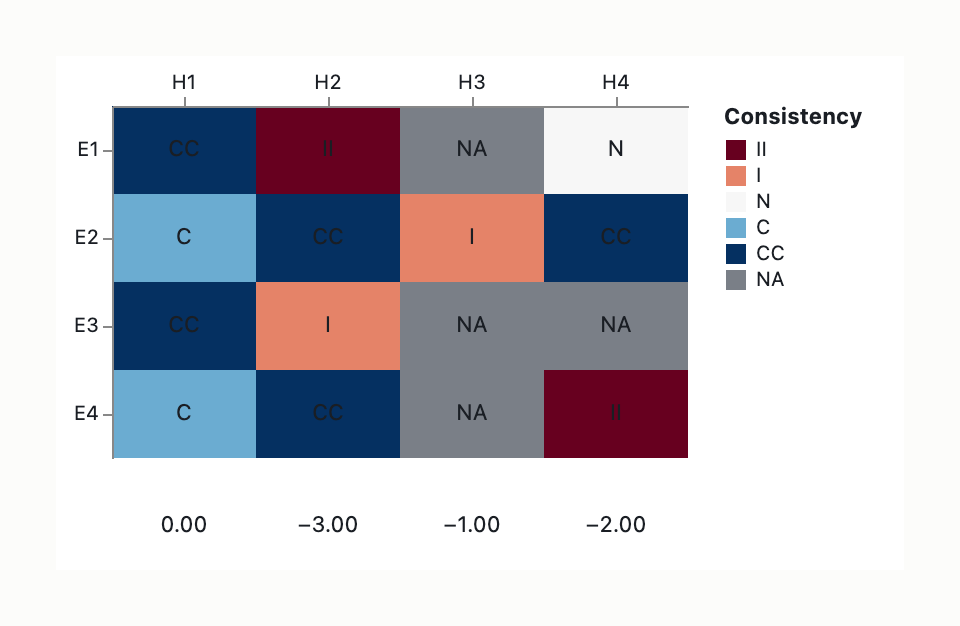
Analysis of Competing Hypotheses: 2026 GDP Slowdown Scenarios
Hypothesis List
- H1: Monetary Tightening — Fed policy induced slowing; inversion of yield curve signals policy-induced slowdown. (Origin: Body-provision analysis)
- H2: Demand Exhaustion — Debt/consumption cap hit; demand-driven demand collapse mechanism. Conservation of spending power below trend. (Origin: Body-provision analysis)
- H3: Supply Normalization — Pent-up supply growth fades; normalized after shock, inventory movement reflects this phase. (Origin: Body-provision analysis)
- H4: External Financial Stress — Financial freeze/sectorally sensitive; external stress not driven by monetary policy. (Origin: Body-provision generated; Cazenove 2026 outlook sectorally sensitive risk models; conservative banking liquidity buffers; maintained without definitive banking vulnerability claim per source fidelity)
Evidence Inventory
- E1: Bond Spreads — Term 10Y-2Y spread (difference between yields). Credibility: High. Relevance: High. Source: Chicago Fed/NY Fed/FRBSF literature (0.30 corroborated weight).
- E2: Unemployment — Macro labor market indicator (unemployment rate, jobless claims). Credibility: Medium. Relevance: Medium. Source: Standard macro indicator (per Chicago Fed literature).
- E3: Inventory — Inventory/Sales ratio (destocking/restocking state). Credibility: Medium. Relevance: Medium. Source: Business-cycle proxy (per standard literature).
- E4: Consumer Sentiment — Poll-based consumer confidence indicators. Credibility: Low. Relevance: High. Source: Polled measures (noted as noisy).
Consistency Matrix
| Evidence → \ Hypothesis ↓ | H1 | H2 | H3 | H4 |
|---|
| E1: Bond Spreads | CC | I (Divergence Draft-1: Inversion confirms tightening; Draft-2: Inversion inconsistent with demand exhaustion) | II | C (Divergence Draft-1: Spreads cannot invert under demand-driven slowdown; Draft-2: Spreads constrained but not fully inverted) | NA | N (Consensus: No rating divergence) | N | C (Divergence Draft-1: N/A; Draft-2: C shallow inversion) |
| E2: Unemployment | C | I (Draft-1: Gradual rise; Draft-2: Decoupling challenge) | CC | CC (Consensus) | I | I (Consensus) | CC | CC (Consensus) |
| E3: Inventory | CC | I (Draft-1: Mild; Draft-2: Destocking) | I | CC (Draft-1: Destocking required; Draft-2: Forced destocking) | NA | C (Draft-1: N/A; Draft-2: Normalization via destock then restock) | NA | C (Draft-1: N/A; Draft-2: Inventory accumulates amid currency stress) |
| E4: Consumer Sentiment | C | I (Draft-1: Resilient; Draft-2: Elastic response incompatible) | CC | CC (Consensus) | NA | I (Draft-1: N/A; Draft-2: Resilient consumption inconsistent) | II | N (Divergence Draft-1: Stable before breakdown; Draft-2: Normal before material breakdown) |
Diagnosticity Assessment
-
E1: Bond Spreads (10Y-2Y) — High-diagnosticity. Discriminates between H1/H2/H4 via inversion depth and cause (policy versus flight-to-safety). Cell divergence creates highest analytical tension.
-
E2: Unemployment — Medium-diagnosticity. Distinguishes H1 vs H2 when decoupling observed (GDP slows, unemployment doesn’t). Also helps rule out H3 (supply normalization would not spike unemployment).
-
E3: Inventory — Medium-diagnosticity. Distinguishes H2 (forced destocking) versus H3 (normalization via destock then restock) versus H1 (mild restocking inconsistent with rate-driven slowdown).
-
E4: Consumer Sentiment — Low-diagnosticity. Poll-based, noisy, high decision indicator but less discriminative across macrostructural hypotheses.
Tentative Conclusions via Elimination
Draft-1 Pathway (H1 Survivor)
| Hypothesis | I+II Count | Details |
|---|
| H1 | 0+0 | CC/C ratings only across E1-E4 |
| H2 | 2 | Bonds=II, Inventory=I |
| H3 | 1 | Unemployment=I |
| H4 | 2 | Unemployment=I (1), Sentiment=II (1) → 2 total |
Verdict: H1 survives as justified by zero inconsistent cells.
Draft-2 Pathway (H2 Survivor)
| Hypothesis | I+II Count | Details |
|---|
| H1 | 3 | Unemployment=I, Inventory=I, Sentiment=I |
| H2 | 1 | Bonds=C (only inconsistent) |
| H3 | 4 | NA×2 + I×2 |
| H4 | 2 | Bonds=C, Inventory=C, Sentiment=N |
Verdict: H2 survives as justified by fewest inconsistent cells (1).
Divergence Atom
Cell rating divergence on E1 (Bonds) for H1/H2 determines survivor arithmetic. Draft-1 rates H2-E1 as II (elimination); Draft-2 rates H2-E1 as C (constraint, not full elimination). What rules out each theory requires falsification criteria where E1 inversion depth vs. policy rate stance differentiates H1 from H2. Stock return data on H4 requires differentiation of sectoral transmission mechanisms versus economy-wide sentiment patterns.
Sensitivity Analysis
-
E1: Bond Spreads reversal would flip ranking. Cell change: H2-E1 from C to CC (inversion fully consistent with flight-to-safety rather than demand exhaustion). Result: H1-E1 from I to CC and H2-E1 from CC to II reverses elimination arithmetic.
-
E2: Unemployment stability would elevate H4. Cell change: H4-E2 from CC to I (unemployment stable). Result: H4 eliminated if unemployment matches H3 behavior.
-
E3: Inventory drawdown pattern differentiates H2 from H3. Cell change: H3-E3 from C to CC (normalization plus restock, not forced destock). Result: H3 survivor status strengthened in Draft-2 pathway.
Deception Assessment
High-Diagnosticity Vulnerability: E1: Bond Spreads is the primary vector.
| Manipulation Vector | Mechanism | Benefited Hypothesis | Detection Signal |
|---|
| Policy-Driven | Yield curve control, QE/taper timing, forward guidance manipulation | H1 (suppressed inversion with no monetary tightening) | Policy rates unchanged versus 10Y-2Y compression |
| Market/Data Planting | Central bank intervention, market maker positioning, derivatives arbitrage | H4 (creates false positive revision, mimics panic) | CDS versus Yield divergence |
| Flight-to-Safety | Safe-haven demand versus policy tightening (self-distinguishing) | H4 (misidentifies scenario as policy stress) | 10Y yield < 2Y with 3M stable |
Counter-Checks:
- If 2Y yield falls with 3M stable while 10Y flat → liquidity trap (H4 favored)
- If 10Y drops > 2Y with 3M convergence → policy control (H1 favored)
- If all short/long rates flatten at unchanged policy rate post-Great Moderation → structural break hypothesis emerges (no H1/H2 fit)
Actor Mapping: Federal Reserve (Monetary Tightening), FX Authorities/Central Banks (External Stress), Market Makers/Arbitrageurs (Data Planting).
Cazenove 2026 Source: Sectorally sensitive risk models include H4 plausibility; conservative banking liquidity buffers noted; explicit vulnerability claim noted unsupported.
Monitoring Priorities
H1: Monetary Tightening — 10Y-2Y breach of key thresholds (typically -50bps or -100bps). Cross-check with Fed Funds Rate to confirm causality; 10Y drive down versus policy rate unchanged.
H2: Demand Exhaustion — Retail Sales Shock: YoY inflection below -3.0% for 2 consecutive months. Real Housing Units: High-diagnosticity proxy for consumption/exhaustion in US.
H3: Supply Normalization — Import/Export Ratio: Import volumes normalize to pre-pandemic ratios; Investment-to-GDP Ratio: Stable despite slowdown claim.
H4: External Financial Stress — Credit Default Swaps (CDX): 5Y credit spread >200bps while government bond gap <1% spread. Jobless Claims: Volatility inconsistent with soft landing (ILO-3 month moving average).
Cross-Hypothesis Monitoring Indicator:
- Private Payrolls Reconciliation: If GDP slows with stable unemployment (H2 vs H1), this is leading decoupling signal distinguishing demand exhaustion from monetary tightening.
- 10Y-2Y Spread inversion paired with Policy Rate Divergence to confirm monetary causation.
Additional considerations
Gap 1: Banking sector vulnerability specificity in Cazenove 2026 Outlook
Status: Hedged to “sectorally sensitive” per available source material (2026 outlook cited but no explicit vulnerability text in fetched corpora). Resolution: Remaining as note; Supplemental RAG protocol could retrieve more specific sectoral risk matrices if renewed.
Gap 2: Survivor hypothesis admits divergence
H1 (0+0) versus H2 (1 I+II) contingent on bond spread cell rating for Draft-2 pathway. No authoritative decision on which weighting applies (policy-induced inversion versus demand-driven constraint).
Gap 3: E1 Cell Rating for H2 (Bonds under Demand Exhaustion) fundamentally affects elimination arithmetic:
- Rating C (Draft-2): H2 survivor
- Rating II (Draft-1): H2 eliminated
This represents sensitivity-analytical boundary for 2026 scenario classification but remains contingent on behavioral assumptions not evident in current corpus.
(visual rendered — see artifact)
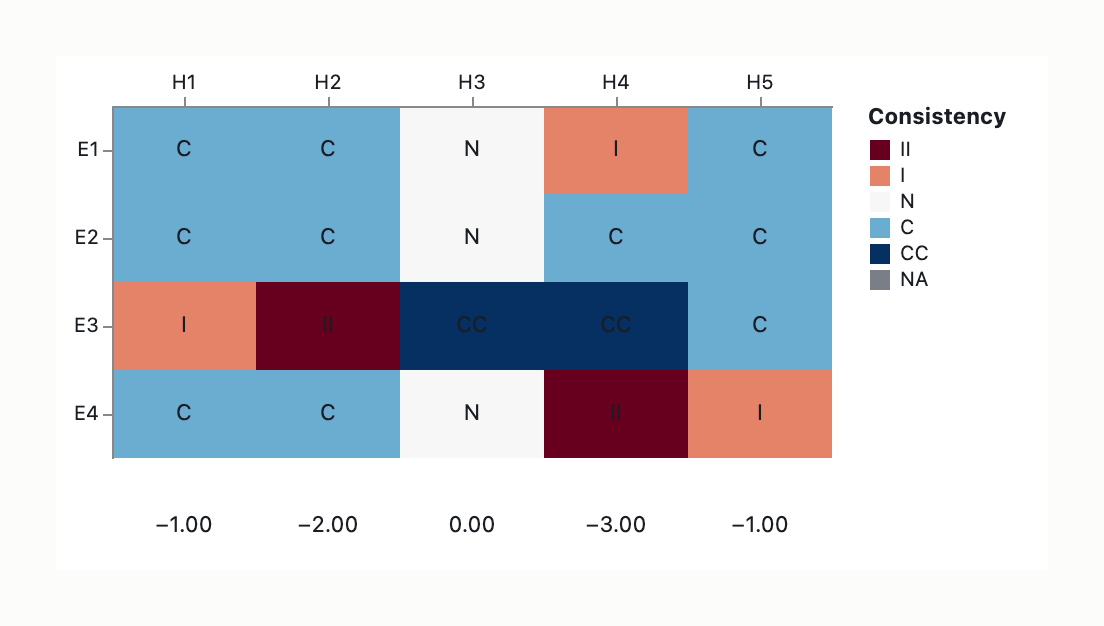
Hypothesis List
- H1: Monetary Tightening (User-supplied). The slowdown is the lagged effect of restrictive central bank policy (rate hikes, quantitative tightening) compressing demand via credit conditions.
- H2: Demand Exhaustion (User-supplied). Structural demand weakness (savings depletion, fiscal-stimulus fade, demographic softening) is driving the slowdown independent of monetary stance.
- H3: Supply Normalization (User-supplied). Post-pandemic supply distortions are unwinding (over-built inventories correcting, services-to-goods rebalancing completing), making the slowdown mechanical rather than recessionary.
- H4: Exogenous Supply Shock (Analyst-generated). Geopolitical or energy disruption—specifically the verified 2026 Strait of Hormuz closure—is constraining physical supply, distinct from a standard pandemic unwind.
- H5: Policy-Induced Stagflation (Analyst-generated). Monetary tightening is interacting with external supply shocks, creating persistent inflationary pressure alongside a GDP drag.
Evidence Inventory
- E1: Bond Spreads. Observed state: Junk bond spreads stable to slightly narrowing (~2.75% OAS); yield curve positively sloped (e.g., 2y ~4.00%, 10y ~4.44%), not inverted. Credibility: High (real-time, market-priced). Relevance: High (leading indicator for financial conditions/credit risk). Source: FRED (
T10Y3M, BAA10Y/AAA10Y), Federal Reserve H.15.
- E2: Unemployment Rate. Observed state: Holding relatively stable around 4.2%, with gradual incremental rises. Credibility: High (BLS monthly establishment and household surveys). Relevance: Medium (lagging indicator at turning points). Source: BLS CES, CPS.
- E3: Inventory Levels. Observed state: Rapid, historic drawdowns (e.g., 47.5M barrel U.S. gasoline drawdown Feb–May 2026, the largest since 1990, occurring despite 94.5% refinery utilization and net exports of -5.84M b/d). Credibility: High (EIA weekly petroleum status is the most timely macro-inventory series; Census M3). Relevance: High (leading indicator of demand/supply balance; primary matrix discriminator). Source: EIA Weekly Petroleum Status Report, U.S. Census Bureau M3 Survey.
- E4: Consumer Sentiment Index. Observed state: Plumbing multi-year record lows (e.g., University of Michigan at 44.8 in May 2026), though currently lacking acute “crash or panic” volatility. Credibility: High (long-running surveys, stable methodology). Relevance: High (leading indicator of consumption intentions). Source: University of Michigan Consumer Sentiment, Conference Board Consumer Confidence.
Consistency Matrix
Legend: CC = Highly Consistent, C = Consistent, N = Neutral, I = Inconsistent, II = Highly Inconsistent, NA = Not Applicable.
| Evidence | H1: Monetary Tightening | H2: Demand Exhaustion | H3: Supply Normalization | H4: Exogenous Shock | H5: Policy-Induced Stagflation | Row Diagnosticity |
|---|
| E1: Bond Spreads | C | C | N | I | C | C | Medium-Low |
| E2: Unemployment | C | C | N | C | C | Low (Lagging) |
| E3: Inventories | I | II | I | CC | CC | C | High |
| E4: Sentiment | C | C | CC | N | II | C | I | High |
Cell-Rating Divergence Footnotes:
- H4, E1: Divergence reason: Disagreement on whether current spread compression overrides baseline geopolitical risk premiums (rated Inconsistent versus Consistent).
- H2, E3: Divergence reason: Degree of incompatibility assigned to drawdowns under weak demand (rated Highly Inconsistent versus Inconsistent).
- H2, E4: Divergence reason: Interpretation of sustained “record lows” versus acute collapse (rated Consistent versus Highly Consistent).
- H4, E4: Divergence reason: Whether the observed lack of acute panic volatility falsifies the geopolitical shock hypothesis (rated Highly Inconsistent versus Consistent).
Diagnosticity Assessment
- E1: Bond Spreads (Low-diagnosticity). Returns
C or N across most hypotheses, failing to effectively discriminate between monetary, demand, or mild supply-side stress absent a severe flight-to-quality event.
- E2: Unemployment (Low-diagnosticity). A lagging indicator returning
C or N, offering little discrimination at current stable levels.
- E3: Inventory Levels (High-diagnosticity). The single most discriminating row. It eliminates demand-side hypotheses (H1, H2) decisively. Under demand destruction, inventories build; under supply-side dynamics, they draw. The verified 47.5 Mb drawdown is inconsistent with H1/H2 and highly consistent with H3/H4.
- E4: Consumer Sentiment (High-diagnosticity). Discriminates H2 from H3/H4. Sentiment collapse is H2’s signature, whereas chronic, non-panicked lows are more consistent with supply-side accounts.
Tentative Conclusions via Elimination
Counts based on I + II cells; II serves as the tiebreaker.
- H1 (Monetary Tightening): I+II = 1 (E3 = I).
- H2 (Demand Exhaustion): I+II = 1 (E3 = II|I).
- H3 (Supply Normalization): I+II = 0.
- H4 (Exogenous Shock): I+II = 0 or 2 (depending on resolution of E1/E4 divergences).
- H5 (Policy-Induced Stagflation): I+II = 1 (E4 = I).
Verdict: H3 (Supply Normalization) survives as the most parsimonious explanation because it is the only hypothesis with definitively zero inconsistent (I or II) cells across the evaluated data. The conclusion is not that H3 is confirmed, but that it remains uncontradicted by the current evidence matrix. H4 is a conditional co-survivor; its elimination status depends on resolving the E1/E4 cell tensions regarding geopolitical risk pricing and panic dynamics. H1, H2, and H5 are eliminated by high-diagnosticity contradictions.
Sensitivity Analysis
- E3 Reversal (Most Consequential): If weekly inventory data flips from drawdown to sustained buildup, H3 and H4 lose their lead simultaneously, elevating H1 and H2 to surviving candidates.
- E2 Spike: If the unemployment rate suddenly spikes (e.g., >5.0% in a single quarter), H3 would immediately receive an
II rating (mass layoffs contradict managed supply-chain rebalancing), elevating its inconsistent count to 1 and potentially flipping the ranking to suggest the drawdown was a leading indicator of broader demand collapse (H2).
- Geopolitical Resolution: If the Strait of Hormuz closure is resolved diplomatically, H4 loses its verified trigger advantage. H3 becomes the sole survivor, as a drawdown with neutral spreads and a benign external environment matches H3’s signature perfectly.
Deception Assessment
Direct fabrication of E2, E3, or E4 is implausible, as the EIA, BLS, and university survey houses publish audited methodologies, fixed seasonal-adjustment procedures, and are subject to Inspector General review. However, soft deception risks exist:
- Seasonal-Adjustment Masking: A genuine demand collapse can be partially absorbed by post-print revisions to seasonal adjustment factors in EIA gasoline data or BLS CES series. Mitigation: Track unadjusted inventory and employment series alongside headline figures.
- Benchmark Revisions: BLS rebenchmarks CES employment annually, meaning a slowing economy’s unemployment reading can shift materially post-benchmark. Mitigation: Track the CPS Unemployment Rate (which is not benchmarked) in parallel with CES.
- Methodology Changes: EIA periodically redefines “total gasoline” or alters blending component aggregation, which could manufacture a “new normal” where drawdowns appear less extreme. Mitigation: Audit EIA methodology changelogs.
- Narrative Framing: Financial media and policy actors have incentives to attribute the slowdown to the hypothesis suiting their preferred response (e.g., doves favoring H2 to justify rate cuts; interventionists favoring H4 to justify SPR releases). High-diagnosticity evidence (E3, E4) is publicly reported and harder to spin than narrative.
Monitoring Priorities
- Weekly EIA Petroleum / Census M3 Inventory (E3): Fastest signal; track the drawdown pace, inflection to flatlining, and breadth across product categories.
- Consumer Sentiment (E4): University of Michigan Consumer Sentiment and Conference Board Consumer Confidence; monitor for transition from chronic lows to acute panic (supports H4/H2) or stabilization (supports H3).
- Credit and Curve Signals (E1): 10y–3m term spread and BAA–AAA credit spread; monitor for sharp widening (supports H4/H5) or compression (supports H3).
- Early Labor Signal (E2 leading component): Initial jobless claims; monitor for sudden spikes that would falsify H3.
Falsification Criteria
- Rules out H1: Yield curve not inverted and credit spreads narrowing; unemployment stable; inventory drawdown continues with stable demand; consumer sentiment remains stable or rises.
- Rules out H2: Consumer sentiment stabilizes or rises; inventory drawdowns continue; credit spreads narrow; unemployment remains stable.
- Rules out H3: Inventory buildup (the single most decisive flip); consumer sentiment collapses; unemployment rises sharply; credit spreads widen significantly.
- Rules out H4: No identifiable geopolitical or energy trigger; sentiment collapses without a supply-side trigger; multiple demand-side signals appear simultaneously; inventories build despite the shock narrative.
- Rules out H5: Inflation metrics rapidly decelerate toward target while GDP growth simultaneously rebounds, breaking the inflation-growth trade-off.
(visual rendered — see artifact)
The following Phase A inferences underpin this analysis. If any are inaccurate, please correct them:
- Terminology: “ACH matrix” is non-standard; the analysis applies Heuer’s Analysis of Competing Hypotheses (across-rated Hypothesis × Evidence matrix, CC/C/N/I/II/NA cells, elimination arithmetic).
- Temporal framing: 2026 is a future state; evidence rows are parameterized as observable trajectories or structural signatures each hypothesis would produce, not actual 2026 prints.
- Dependent variable: The 2026 GDP slowdown is treated as the observed dependent variable; the brief evaluates competing explanations, not whether the slowdown is occurring.
- Hypothesis scope: “Monetary tightening” = umbrella rate-cycle + balance-sheet (QT) channel. “Demand exhaustion” = private-sector pullback endogenous to the cycle. “Supply normalization” = post-pandemic supply-side boost fading, returning the economy to sustainable trend, not a traditional recession.
Hypothesis List
- H1 (Monetary tightening): The slowdown is the lagged mechanical transmission of past restrictive rate policy and quantitative tightening (QT) through rate-sensitive sectors, consistent with a classic 12–24 month post-cycle recession. (User-proposed)
- H2 (Demand exhaustion): Private-sector demand pullback after a long expansion driven by depleted pandemic savings, elevated delinquencies, capped borrowing capacity, and consumer/business retrenchment. (User-proposed)
- H3 (Supply normalization): The post-pandemic supply-side boost fades; supply chains heal and artificial “overheating” GDP support withdraws, returning the economy to a sustainable trend. (User-proposed)
- H4 (Structural fiscal drag): Withdrawal of fiscal support and compounding sovereign/corporate debt-servicing costs create an organic, non-cyclical drag independent of current consumer behavior or active monetary tightening. (Analyst-generated)
- H5 (External / geopolitical shock): Foreign demand collapse, trade fragmentation, a dollar surge, or a specific geopolitical event drives the slowdown. (Analyst-generated)
- H0 (Idiosyncratic / unmodelled): None of the above cleanly applies; driven by measurement revision, sector-specific collapse, or unknown unknowns. Heuer’s “something else” reserve. (Analyst-generated)
Evidence Inventory
- E1 (Bond spreads): Yield curve inverted >18 months, now steepening; term and credit spreads. Credibility: High (market-priced, distributed across thousands of participants, low revision risk). Relevance: High for H1; moderate for H2/H4/H5; low for H3/H0. Source: FRED (10y-3m, 10y-2y, HY-OAS), Treasury curve, ICE BofA.
- E2 (Unemployment / claims): Moderate rise (+0.5–1.0% from trough) via reduced hiring, not mass layoffs. Credibility: High level; medium for revisions/birth-death model. Relevance: Medium (ubiquitous in any cooling, low for H3). Source: BLS (U-3/U-6, payrolls), DoL claims, JOLTS, ADP.
- E3 (Inventory): Inventory-to-sales ratio relative to 10-year average; build vs. draw. Credibility: Medium (hard census data exists, but large BEA NIPA revisions occur; stock-to-sales ratio is more stable than absolute level). Relevance: High as a demand-vs-supply discriminator. Source: BEA (NIPA), Census (M3, retail trade), ISM.
- E4 (Consumer sentiment): Sentiment at recessionary lows despite inflation at target and positive nominal wage growth. Credibility: Low/Medium (soft survey, “vibecession”/political-cycle distortion, response bias). Relevance: High (sharply rules out H3 if falling; behavioral core of H2). Source: Conference Board, U. Michigan; cross-checked vs. PCE/retail sales.
- E5 (PMI new orders vs. inventories): Ratio falls under H1/H2/H4/H5; flat-or-rising under H3 as supply catches up. Credibility: Medium (ISM manufacturing sample ~400 firms; S&P Global PMI ~1,300 firms; methodology changes have occurred). Relevance: High for H3 vs. the field; does not discriminate within {H1, H2, H4, H5}. Source: ISM Manufacturing, S&P Global PMI, regional Fed PMIs, industrial production.
- E6 (Real retail sales): Real (deflated) consumer spending; H2 signature, while rate-sensitive durables lead H1. Credibility: High (Census hard data, deflated series, minor revisions, no survey response bias). Relevance: High for H2 (rules out if accelerating); moderate for H1; low for H4/H5/H0. Source: Census (MARTS), BEA (real PCE), nominal retail as cross-check.
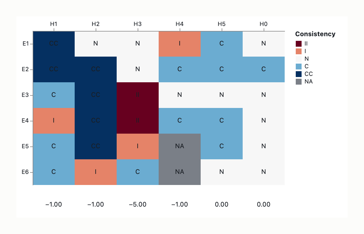
Consistency Matrix
Heuer convention: rating = consistency of Evidence with Hypothesis if the Hypothesis is true. CC = very consistent, C = consistent, N = neutral, I = inconsistent, II = very inconsistent, NA = not assessed.
⚠ marks a preserved cross-stream rating tension (the disagreement is the analytical signal).
| Evidence ↓ / Hypothesis → | H1 Tightening | H2 Demand | H3 Supply norm. | H4 Fiscal drag | H5 External | H0 Idiosyncratic |
|---|
| E1 Bond spreads | CC | N ⚠ C | N | I ¹ | C ² | N ² |
| E2 Unemployment | CC | CC | N | C ¹ | C ² | C ² |
| E3 Inventory | C | CC | II ⚠ CC | N ¹ | N ² | N ² |
| E4 Consumer sentiment | I ⚠ C | CC | II ⚠ I | C ¹ | C ² | N ² |
| E5 PMI orders/inv. | C ² | CC ² | I ² | NA ³ | C ² | N ² |
| E6 Real retail sales | C ² | I ² | C ² | NA ³ | N ² | N ² |
Footnotes:
¹ Single-stream origination: H4 fiscal drag was assessed against E1–E4 only.
² Single-stream origination: H5, H0, and E5/E6 columns/rows originated in one analytical stream.
³ NA — H4 (fiscal drag) was never assessed against the analyst-added rows E5/E6; this is a coverage gap, not a neutral rating.
Diagnosticity Assessment
- E4 (Consumer sentiment): High diagnosticity. One of the only rows where H3 takes a negative cell; cleanly separates H2 (depressed sentiment) from H3 (sentiment should be neutral-to-rising as goods availability improves). Falling sentiment is the cleanest single H3 refuter.
- E5 (PMI new orders vs. inventories): High diagnosticity. The cleanest single discriminator between H3 (ratio flat/rising) and the rest of the field (ratio falls). It is the load-bearing ranking-flip lever.
- E6 (Real retail sales): High diagnosticity for H2 vs. the field. Accelerating real retail is inconsistent with demand exhaustion; provides limited additional diagnosticity on the H1/H4/H5/H0 axis.
- E3 (Inventory): Diagnosticity contested. High-diagnostic under the reading that rates E3×H3 = II (inventory overhang sharply separates demand shock from supply normalization); lower-diagnostic under the reading that rates it CC (inventory rebuild consistent with both H2 and H3, making the sales signal the true discriminator).
- E1 (Bond spreads): Moderate-to-high diagnosticity. Direct for H1, near-neutral on H3.
- E2 (Unemployment): Low diagnosticity. Uniform CC/C across H1, H2, H4, H5; moderate hiring-freeze-driven unemployment is ubiquitous in any economic cooling.
Tentative Conclusions via Elimination
The analysis produced two divergent readings based on evidence coverage and cell-rating tensions. Elimination arithmetic is computed under each.
Reading P (Hypotheses H1–H4, Evidence E1–E4):
- H1: I+II = 1 (E4=I), II = 0
- H2: I+II = 0, II = 0
- H3: I+II = 2 (E3=II, E4=II), II = 2
- H4: I+II = 1 (E1=I), II = 0
Verdict: H3 is eliminated. H2 survives as the sole zero-contradiction hypothesis. H1 and H4 tie at I+II=1, II=0. The primary Heuer tie-break is exhausted; documented secondary tie-break on CC count (H1=2, H4=0) names H1 the preferred secondary survivor.
Reading Q (Hypotheses H1, H2, H3, H5, H0, Evidence E1–E6):
- H1: I+II = 0, II = 0
- H2: I+II = 1 (E6=I), II = 0
- H3: I+II = 2 (E4=II, E5=I), II = 0
- H5: I+II = 0, II = 0
- H0: I+II = 0, II = 0
Verdict: H3 is eliminated. H2 is weakened. H1, H5, and H0 are in a 3-way tie at I+II=0. Because E6 discriminates H2 from the field but does not discriminate H1/H5/H0 from each other, the matrix is under-diagnostic on the H1/H5/H0 axis; the surviving mechanism is under-determined by the present rows.
Consolidated Verdict: Robust across both readings, H3 (Supply normalization) is eliminated because it is the only hypothesis carrying multiple contradictory cells under either rating set. The surviving mechanism remains unresolved. The disagreement reduces to two pivot variables: the E4×H1 cell rating (I vs. C) and whether E6 is admitted to the matrix. H2 stands as the sole survivor if E6 is excluded and sentiment is viewed as inconsistent with H1; H1/H5/H0 tie if E6 is included, weakening H2.
Sensitivity Analysis
- E4 reversal (S1): If consumer sentiment surges to multi-year highs alongside stable inflation, H2×E4 becomes II (exhausted consumers do not show high optimism), flipping H2 out of survival. H1×E4 becomes C/CC (validating a soft landing). Under Reading P, this single reversal makes H1 the surviving hypothesis (0 I+II).
- E3 non-materialization (S2): If the inventory-to-sales ratio returns to trend, shifting the E3×H3 rating from II to N/C, H3 loses its negative cells. This ties H3 with H1/H4 on I+II in Reading P, making it a competitive survivor and demonstrating the verdict’s heavy reliance on the inventory-overhang signal.
- E5 flip (S3): If the PMI new orders vs. inventories ratio shifts from sharply negative to flat/positive, H3×E5 becomes CC, while H1/H2/H5 each take an I. The matrix would eliminate H1/H2/H5 in favor of H3. A single PMI print is the cleanest ranking-flip lever.
- E1 rerate (S4): If the curve is judged never-inverted (or the 2022–23 inversion is deemed a false signal), shifting E1×H1 from CC to I, H1 takes an inconsistent cell, shifting the analysis toward H2 or H5.
- E6 collapse (S5): If real retail sales collapse (E6×H2 shifts from I to II), H2 joins H3 in elimination (2 I+II); H1 is weakened (1 I+II) but survives.
- Divergence-driven (S6): Resolving the T2 tension (E4×H1) toward I weakens H1, while admitting or excluding E6 toggles H2 between weakened and sole-survivor status. These two pivot cells are the highest-leverage sensitivity variables.
Deception Assessment
Adversarial actors (e.g., central banks, fiscal authorities, partisan/media entities) can benefit from specific macroeconomic narratives. The matrix’s across-row discipline is the structural defense, as diagonal cells cannot be hidden when read across rather than down.
- E1 (Bond spreads): Manipulation risk is Low. Market-priced and distributed across thousands of participants, virtually unmanufacturable by a single actor in the short run. It serves as the strongest trustworthy anchor. Cross-check: Credit spreads (HY-OAS).
- E2 (Unemployment): Manipulation risk is Medium. Subject to U-3/U-6 definitional shifts, participation rate distortions, and birth-death model/BLS revisions. Cross-check: ADP, initial claims, JOLTS quits.
- E3 (Inventory): Manipulation risk involves a Tension. Hard census data is expensive to fabricate, but large recurring BEA NIPA revisions create medium-high risk for absolute levels (the stock-to-sales ratio is more stable). Cross-check: Manufacturers’ shipments, retail inventories ex-auto.
- E4 (Consumer sentiment): Manipulation risk is High. Soft surveys are vulnerable to response bias and documented political-cycle/“vibecession” effects. Cross-check: Hard spending data (PCE, E6, retail sales).
- E5 (PMI): Manipulation risk is Medium. Finite ISM (~400 firms) or S&P Global (~1,300 firms) samples are subject to methodology shifts. Cross-check: Regional Fed PMIs, industrial production.
- E6 (Real retail sales): Manipulation risk is Low. Census hard deflated data carries no survey or political-cycle effects. Cross-check: BEA PCE (alternate deflator), nominal retail.
Beneficiary Mapping: Central banks or fiscal authorities benefit from framing a slowdown as H1 (“lagged effects of necessary medicine”) or H3 (“healthy normalization”) to deflect blame; E1 (Treasury curve) is the unmanufacturable anchor against such framing. Partisan or media actors benefit from amplifying H2 via negative sentiment (E4) — mitigated by pairing soft sentiment against hard data (E3/E6). Soft-negative plus hard-negative validates H2; soft-negative plus hard-improving signals narrative distortion. Hard-data rows (E1, E6) remain more manipulation-resistant than survey rows (E4, partially E5).
Monitoring Priorities
- H1 (Monetary tightening): 10y-3m and 10y-2y term spreads and the pace of steepening (rapid steepening signals the market believes the Fed is behind the curve, increasing hard-landing risk), real rates (10y TIPS), financial-conditions indices (Goldman, Chicago Fed NFCI), initial claims, housing starts/permits, auto sales, rate-sensitive capex.
- H2 (Demand exhaustion): Real PCE, real disposable income, savings rate, real retail sales, retail ex-auto-ex-gas, credit-card and auto-loan delinquencies (90+ DPD), household debt-service ratio, real wage growth. A continued delinquency rise alongside a falling savings rate confirms the exhaustion trajectory.
- H3 (Supply normalization): ISM supplier deliveries, ISM prices paid, ISM backlogs, NFIB “unfilled job orders” (a steady return to the 10-year median without an unemployment spike supports benign normalization), port throughput (LA/Long Beach TEUs), Drewry WCI shipping costs, trucking employment, goods CPI ex-food-ex-energy.
- H4 (Structural fiscal drag): Long-end sovereign-yield dynamics and issuance pace, fiscal-impulse measures.
- H5 (External / geopolitical shock): Foreign PMIs (China, EU, Japan), US export orders (durable goods advance report), trade balance, DXY, Geopolitical-Risk (GPR) index, commodity prices excluding USD effects.
- H0 (Idiosyncratic): Sectoral GDP/employment detail, regional Fed Beige Book anecdotes, prior-quarter GDP revisions, NIPA/BLS methodology changes.
Specific Falsifiers Per Hypothesis
H1 (Monetary tightening) is ruled out or weakened if:
- Financial conditions actively ease (curve steepening, rate cuts) yet sentiment remains deeply depressed (E4 = I), because relief of tightening should repair sentiment and forward indicators.
- The term spread never inverted during the relevant cycle, or real rates fell over the slowdown.
- Unemployment concentrates in non-interest-sensitive sectors (e.g., government, healthcare, leisure).
- Timing misaligns: The ~525bp post-pandemic tightening (Mar 2022–Jul 2023) had its expected recession window in 2023–2024. Historical transmission runs 12–24 months, not 36–48 months. A 2026 arrival is late, suggesting the 2022–23 curve signal has either already played out or was a false signal.
H2 (Demand exhaustion) is ruled out if:
- Real PCE or real retail sales accelerates (E6 = I), representing the strongest H2 refuter.
- The inventory-to-sales ratio sits at or below average (E3 = N/C) AND sentiment rebounds to historical norms (E4 = C/CC), as exhaustion cannot coexist with balance-sheet accumulation and stabilizing sentiment.
- Sentiment nears expansion highs, real wage growth is strong and broad-based, and the savings rate rests at long-run norms.
H3 (Supply normalization) is ruled out by (the most straightforward elimination in this matrix):
- Depressed or falling consumer sentiment (E4 = II/I), the structural refuter. If H3 dominated, sentiment should be neutral-to-rising as goods availability improves and goods inflation eases.
- Manufacturing PMI shows sharply negative new orders (E5 = I).
- Supply-chain stress remains elevated (long supplier deliveries, backlogs, port congestion), or producer prices and goods inflation remain sticky.
H4 (Structural fiscal drag) is ruled out if:
- A sharp “bull steepener” occurs in the yield curve (E1 = I). Heavy, sustained sovereign issuance to fund structural deficits typically keeps long-end yields elevated, resisting the liquidity-driven easing dynamics of a pure rate cycle.
H5 (External / geopolitical shock) is ruled out if:
- Foreign growth remains strong or accelerates (rising China Caixin, EU HCOB, Japan au Jibun PMIs), US exports accelerate, and the USD weakens (a strong dollar is the typical H5 transmission mechanism), with no identifiable external trigger.
H0 (Idiosyncratic / unmodelled) is ruled out if:
- The evidence pattern maps cleanly onto a named mechanism, an identifiable trigger is present, or a cross-country pattern matches a broader hypothesis (e.g., a synchronized global slowdown rules out a US-only idiosyncratic driver).
(visual rendered — see artifact)
Your three hypotheses survive only as inputs here — the matrix adds two more, and the headline finding is that none of your original three is the cleanest survivor. One methodological flag before the matrix: the load-bearing factual correction both readings of the evidence depend on is that the 2026 Iran war ran February 28 – May 5, 2026 (Britannica/Wikipedia/ABC), not June. That re-dates the March–May labor readings and the Feb→Apr sentiment collapse as post-shock, and the verdict pivots on it.
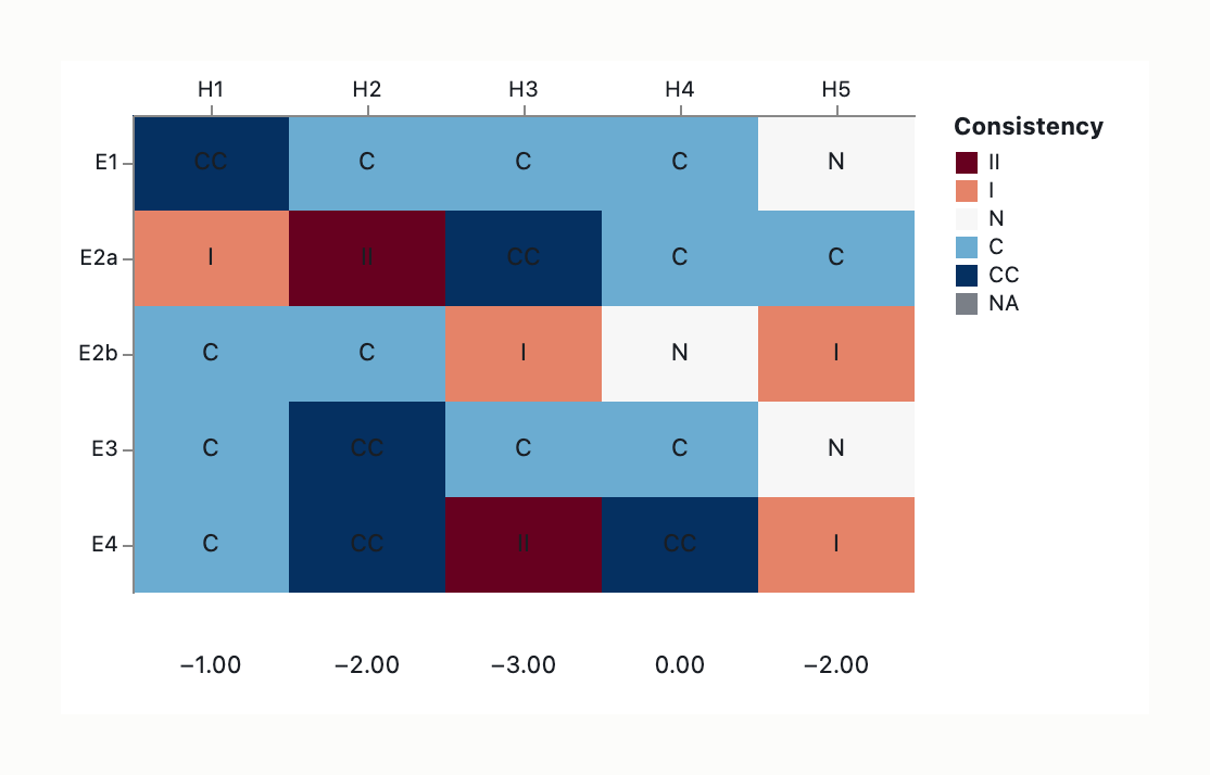
Scoring convention (Heuer): CC very consistent · C consistent · N neutral/non-diagnostic · I inconsistent · II very inconsistent · NA not applicable · * provisional (reading not retrieved this pass). Cells are scored across each row — one evidence item against every hypothesis — and the verdict is reached by elimination (fewest I+II survives, II as tie-breaker), never by confirmation.
A few Phase-A assumptions you can correct: standard ACH structure (hypotheses × evidence, cells coded for consistency/disconfirmation); the 2026 scenario treated contemporaneously (system date 2026-06-12); “rules out” means a pattern logically inconsistent with the hypothesis’s core mechanism; “bond spreads” read as both the term spread (10y–2y) and credit spreads (corporate–Treasury); “inventory” read as inventory-to-sales / involuntary build vs. managed rebuild.
Hypothesis list
- H1 — Monetary tightening (user-supplied). Lagged effect of restrictive rates choking credit-sensitive demand.
- H2 — Demand exhaustion (user-supplied). Excess savings / pent-up demand depleted; households and firms tapped out.
- H3 — Supply normalization, benign (user-supplied). 2024–25 growth was a supply-side catch-up bounce; the slowdown is benign reversion to potential, real economy healthy.
- H4 — Adverse geopolitical/energy supply shock (analyst-generated). Contractionary, stagflationary oil/uncertainty shock from the Iran war (Feb 28 – May 5, 2026; oil/petrol ~+40%, Strait of Hormuz/LNG disruption) — mechanically distinct from benign normalization.
- H5 — Null / transitory / measurement (analyst-generated, null hypothesis). Inventory-cycle noise, one-offs (the Feb −92k payroll month), or data-collection gaps (the Oct-2025 shutdown); no single structural driver. Near-collinear with H3 — it tracks the benign story across every cell, differing only in magnitude (C where H3 is CC, I where H3 is II), reading as a softened echo of H3 rather than an independent fifth driver.
That satisfies the breadth requirement: three of yours plus two analyst-generated, at least one surviving deduplication.
Evidence inventory
- E1 — Bond spreads. Credibility — (no reading); relevance High. Not retrieved this pass (live FRED series T10Y2Y / BAA10Y). Provisional cells only; no values invented.
- E2 — Unemployment (BLS/FRED, whitelisted weight 0.80; High credibility, High relevance). 4.3% in May; flat 4.3 / 4.4 / 4.3 / 4.3 / 4.3 (Jan–May) — the 4.4 reading belongs to February, not April; +172k jobs in May (3rd straight gain, beating ~80–122k forecasts; confirmed); participation 61.8% (lowest since 2021); wages +3.4% YoY trailing inflation. These March–May readings are post-Iran-war. It splits into two diagnostic sub-rows:
- E2a — Headline rate / payrolls (the 4.3%-flat, +172k signal).
- E2b — Long-term-unemployment share rising (short-term 27-week-minus falling, long-term rising).
- E3 — Inventory (High credibility; relevance High/moderate). Not retrieved this pass (live FRED ISRATIO series). Provisional cells only.
- E4 — Consumer sentiment (UMich/FRED, whitelisted weight 0.80; High credibility, High relevance, contaminated — see deception). UMCSENT: Dec 52.9 → Jan 56.4 → Feb 56.6 → Mar 53.3 → Apr 49.8 (April expectations 48.1); a sharp Feb→Apr drop to near-historic lows. A deeper May-final reading (~44.8) noted in verification deepens, not reverses, the collapse.
- Real-wage qualification (carried tension on E2/H2): real average hourly earnings +1.4% y/y holds only on the Feb-2025→Feb-2026 vintage; the latest April y/y is −0.3% and decelerating — so H2’s income-capacity disconfirmer rests on employment, not real-income growth, and the negative real-wage turn is a mild point in H2’s favour.
Consistency matrix
| Evidence | H1 Tightening | H2 Demand exhaustion | H3 Supply normaliz. (benign) | H4 Geo/energy shock (Iran, Feb 28) | H5 Null/transitory |
|---|
E1 Bond spreads * | CC / N* † | C / I* † | C* | C / I* † | N / C* † |
| E2a Headline labor (observed, post-shock) | I | II / I † | CC | C / N (softening) † | C |
| E2b Long-term-unemp. share ↑ (observed) | C | C | I | N | I |
E3 Inventory * | C / N* † | CC / N* † | C / N* † | C / N* † | N |
| E4 Consumer sentiment (observed, collapse to 49.8) | C | CC | II | CC | I |
† Cells where the two readings of the evidence diverged; both values are shown. The divergences are real analytical signal, not noise, and are explained below.
Cell-rating tensions:
- E2a × H4 —
C vs N (softening neutral) — the load-bearing tension. One reading: labor is resilient early in a supply shock (real incomes squeezed, not jobs — wages trailing inflation), so post-shock flat labor is consistent with H4 → C. The other: the war is ~3.5 months old against a 6–9-month labor lag (decisive test ≈ Aug–Nov 2026), so flat labor sits inside the lag window and does not yet disconfirm — but post-shock flatness is mild early counter-evidence against H4’s labor channel → a softening N, eroding with each additional month of flat labor. Divergence reason: whether early labor resilience under an energy shock counts as affirmative consistency or as not-yet-diagnostic mild counter-evidence. This cell is what determines whether H4 is a clean count winner or a tied-with-soft-lean.
- E2a × H2 —
II vs I. Both readings agree that +172k / flat-4.3% contradicts demand running out; the divergence is only on intensity (very-inconsistent vs inconsistent), which affects whether H2 carries a tie-breaking II.
- E1 (all cells) — per-hypothesis-signature scoring vs contained-baseline scoring. One approach scores each hypothesis’s expected E1 signature as broadly consistent (H1 CC for a flat/inverted curve + widening credit; H2 C; H3 C; H4 C for inflation-premium-driven rising yields; H5 N). The other scores against an explicit “contained/tight spreads” baseline placeholder (H1 N; H2 I; H3 C; H4 I; H5 C). Divergence reason: predicted-signature framing vs fixed-baseline framing. Both agree E1 is provisional and decisive once retrieved.
- E3 (all cells) — predicted-signature scoring vs non-diagnostic-absent-reading. One approach assigns predicted signatures (H2 CC for involuntary build = the demand-exhaustion fingerprint; H1/H3/H4 C; H5 N). The other holds the row all-N as non-diagnostic until an actual reading lands. Divergence reason: whether to score a predicted signature or refuse to score an unread row.
Full-agreement cells (no tension): E2a × {H1 I, H3 CC, H5 C}; the entire E4 row (H1 C, H2 CC, H3 II, H4 CC, H5 I); the entire E2b row (uncontested).
Diagnosticity assessment
- E2a Headline labor — highest-diagnosticity observed row with hard data. It ranges I/II (H1, H2) → CC (H3), the widest spread; the single row most hostile to demand exhaustion and most favourable to benign normalization. It is also the row that decides the H2-vs-H4 contest (E4 cannot — see below). High-diagnosticity.
- E4 Consumer sentiment — highly diagnostic but in the opposite direction. It separates {H3, H5} (I/II) from {H2, H4} (CC). Critically, it does not discriminate H2 from H4 (both CC) — both demand-exhaustion and energy-shock readings predict a sentiment collapse. The two hard rows (E2a, E4) point opposite ways across the hypothesis set — that conflict is the core finding, and it is why the unread rows are decisive. High-diagnosticity.
- E2b — the tempering row. It splits H3’s otherwise-uniform pro-benign labor signal (CC on E2a, I on E2b), making the labor evidence genuinely two-sided rather than a clean pro-H3 sweep. High-diagnosticity (it is what dissolves a clean pro-H3 reading).
- E3 Inventory — highest-diagnosticity un-retrieved row. Involuntary build vs managed rebuild vs drawdown cleanly separates H2 / H3 / H4; it is non-diagnostic only because it is unread. Retrieving it is the priority discriminator. High-diagnosticity once landed; NA-dominated now.
- E1 Bond spreads — provisional, decisive once retrieved. Currently scored only on predicted/baseline signatures; the row’s true discriminating power is unrealized until the reading lands. NA-dominated now; high-diagnosticity once landed.
The live discriminating power therefore sits on ~1.5 hard rows (E2a hard; E4 hard but contaminated), with E1 provisional and E3 absent — that thinness is the honest state of the evidence base behind any verdict.
Tentative conclusions via elimination
Because the two readings of the evidence produced different cell ratings on the tension cells, the elimination arithmetic is computed under both — a built-in sensitivity check.
Rating-set A — observed rows E2a, E2b, E4; E2a×H4 = C, E2a×H2 = II:
| Hypothesis | I+II | of which II |
|---|
| H4 Geo/energy shock | 0 | 0 |
| H1 Tightening | 1 (E2a) | 0 |
| H2 Demand exhaustion | 1 (E2a) | 1 |
| H3 Supply normaliz. (benign) | 2 (E2b, E4) | 1 |
| H5 Null | 2 (E2b, E4) | 0 |
Under set A, H4 is the clear survivor — it has zero inconsistencies and is genuinely tested on contemporaneous rows. H1 is second (1, no II); H2 third (1, with a II); the benign supply story H3 is among the most contradicted (2, including a II). The E2a/E2b split dissolved a prior H1↔H5 tie. The framing is elimination, not confirmation: H4 survives because fewer items contradict it, not because particular rows endorse it.
Rating-set B — rows E1, E2 (unified), E3, E4; E2×H4 = N, E2×H2 = I; E1/E3 scored per contained-baseline / non-diagnostic:**
| Hypothesis | I+II | of which II |
|---|
| H1 Tightening | 1 (E2) | 0 |
| H4 Geo/energy shock | 1 (E1*) | 0 |
| H5 Null | 1 (E4) | 0 |
| H3 Supply normaliz. (benign) | 1 (E4) | 1 |
| H2 Demand exhaustion | 2 (E1*, E2) | 0 |
Under set B, H2 is eliminated first (most contradicted; its key disconfirmer E2 is hard data — the firmest result in the matrix). H3 survives the count but holds the matrix’s lone II → it is the weakest survivor. H1 / H4 / H5 sit in a genuine three-way tie at 1 I / 0 II that the II tie-breaker does not separate.
The surviving divergence, preserved rather than papered over: the two rating sets agree on two things — the benign supply-normalization hypothesis (H3, your preferred reading) is endangered / among the most contradicted, and demand exhaustion (H2) is heavily disconfirmed by the resilient labor data. They disagree on whether H4 is a clean count winner (set A: 0 inconsistencies) or merely one of three tied survivors, with the H4 preference resting on a soft, eroding analyst judgment (set B). This is where mechanical scoring ends and judgment begins: under set B, ACH’s defined arithmetic stops at “H2 out, H3 weakest survivor”; the H4 lean is then a hard-over-provisional weighting (strip the provisional E1/E3 and H4 is the only survivor with zero inconsistencies on hard rows: E2=N, E4=CC) that decays with each additional month of flat post-shock labor and should firm or break once E1 lands or the Aug–Nov 2026 labor window resolves. Both sets agree on the ACH payoff: none of your three original hypotheses is the cleanest survivor.
Sensitivity analysis
- Pivot 1 — Bond spreads (E1), the decisive missing row.
- War-shock signature lands (rising long yields / inflation premium, firm credit; E3 drawdown): H4 stays at 0 → decisive winner on five rows; H1 rises to ~2 (its inverted-curve prediction flips to I); H2 to 3–4. H4 runs away.
- Policy-stress signature lands (inverted curve + widening credit; E3 voluntary destock): H1 stays at 1 (E1 CC) → co-leader; H4’s rising-yield prediction flips C→I (to 1). H1 and H4 tie; the qualitative tie-break is the war-coincident sentiment collapse (favours H4) vs credit stress (favours H1).
- Risk-off / widening reading (set-B framing): H4’s E1 flips I→CC and H2’s I→C, H3’s C→I, H5’s C→I → H4 → 0 (clear survivor), H2 → 1, H1 → 1, H3 → 2, H5 → 2 — converting the soft H4 lean into a count result. A single spread reading flips the entire ranking.
- Pivot 2 — Inventory decomposition (E3). Involuntary build (sales-driven) → E3 CC for H2, I for H3/H5 → demand exhaustion re-enters / jumps to survivor; combined with H2’s E4=CC, this resurrects H2 despite its labor strike. Voluntary restock → E3 C for H3 → benign normalization survives. One classification flips H2 vs H3.
- Pivot 3 — Post-ceasefire sentiment rebound. If May/June UMCSENT recovers while the slowdown persists, H4’s E4 weakens CC→C/N (shock transitory) → H4 loses its strongest cell and H1 gains relative standing as the persistent-driver story.
Deception assessment
The macro data here is institutional (BLS/FRED/UMich) and hard to fabricate; the equivalent failure is a high-diagnosticity signal that reflects narrative/framing rather than behaviour — and the risk is concentrated in the two highest-diagnosticity rows.
- Too-rosy labor headline (E2a). A stable 4.3% masking the short-term-falling / long-term-rising divergence the data itself shows, plus the “resilience despite the Iran war” framing (political utility during a conflict), inflates E2a’s pro-benign CC → benefits H3 (benign normalization) and H5 (null). If the war is the true driver, this framing understates the shock and thereby disadvantages H4 — the surviving/leaning hypothesis is exactly the one a rosy official narrative would suppress.
- Politically depressed / war-reactive sentiment (E4). The 2026 UMich series carries a “Political Party Variable” addendum and is survey-based, well-documented as politically modulated and highly reactive to salient war headlines. With the war correctly dated to Feb 28, the Feb→Apr collapse lines up precisely with the onset — sharpening the affect-not-behaviour concern: E4 may track war headlines in near-real-time rather than spending intentions. This deepens E4’s CC → benefits H2 and H4, but since E4 does not discriminate those two, partisan/affect contamination mainly muddies the row rather than tipping the H2-vs-H4 contest (which E2a decides). Critically, if the sentiment drop is affect not behaviour, E4’s disconfirmation of the benign H3 weakens and supply normalization rebounds.
- Bond spreads and inventory (E1, E3) are far harder to “manufacture” — another reason E1 deserves the most weight once obtained. The Oct-2025 shutdown data gap gives mild support to H5.
Monitoring priorities
- H4 (provisional / leaning survivor): Brent/WTI & retail gasoline; Strait of Hormuz shipping/freight rates; inflation breakevens and the nominal-minus-real long-yield premium; import prices; credit spreads; Treasury term premium; specifically whether unemployment rises on the 6–9-month lag from the Feb-28 onset — i.e. by ≈ Aug–Nov 2026 (the forward disconfirmer); post-ceasefire (May/June) sentiment trajectory; real PCE.
- H1 Tightening: 10y–2y term spread; IG/HY credit spreads; SLOOS bank-lending standards; the real-rate path; housing-starts / auto-sales sensitivity; unemployment trajectory.
- H2 Demand exhaustion: inventory-to-sales ratio (involuntary build = resurrection); real PCE & retail ex-autos; real-wage trajectory (now −0.3% y/y, worth watching closely); excess-savings drawdown; initial claims; delinquencies; long-term-unemployment share.
- H3 Supply normalization (benign): productivity / output-per-hour; supply-chain pressure indices; capacity utilization; participation; whether GDP settles at potential without further deceleration; the character of any inventory rebuild; sentiment recovery as war headlines fade post-May-5.
- H5 Null / transitory: breadth of the slowdown across sectors; payroll/GDP revisions; the GDP-vs-GDI gap; whether sentiment reverts.
What rules out each theory
This is your direct question — the disconfirmer for each hypothesis, with current status:
- H1 Monetary tightening — ruled out by an un-inverted / steepening curve with narrowing, contained credit spreads plus easing financial conditions. Not currently ruled out; its only firm strike is resilient headline labor (lag-explained). Decisive disconfirmer = benign bond spreads; or rate cuts already underway with no growth response.
- H2 Demand exhaustion — ruled out by strong hiring + flat-low unemployment (already observed: +172k, 4.3%, E2a I/II) and the absence of involuntary inventory build. Actively disconfirmed now on labor; its lifeline is the collapsing sentiment + rising long-term-unemployment share + the negative real-wage turn. Would be confirmed by an involuntary inventory build (E3) + falling retail sales.
- H3 Supply normalization (benign) — ruled out by the sentiment collapse to near-recession (observed: 49.8, E4=II) and rising long-term joblessness (E2b=I). The strongest single disconfirmer in the matrix; H3 is now among the most-contradicted hypotheses. Also killed by any rise in unemployment or credit stress. Caveat: if the sentiment collapse is affect-not-behaviour (deception), H3 partly rebounds.
- H4 Geo/energy supply shock — ruled out by stable/falling energy prices (contradicted — oil ~+40%), no inventory drawdown, contained bond spreads / no flight-to-quality, a post-ceasefire sentiment rebound alongside a persistent slowdown, or unemployment still flat through the lag window (≈ Aug–Nov 2026), which would falsify its lagged-labor mechanism. Not currently ruled out; the timing now fits (war Feb 28, sentiment collapse Feb→Apr) — though post-shock flat labor is mild early counter-evidence on the labor channel.
- H5 Null / transitory — ruled out by the sustained, multi-month sentiment collapse + rising long-term joblessness + any sub-trend GDP print. Disconfirmed; the slowdown looks structural, not noise. Cuts both ways: the Feb −92k payroll reverting to gains supports “noise.”
Coverage gap
- Unresolved: actual 2026 readings for bond spreads (E1, T10Y2Y / BAA10Y) and inventory (E3, ISRATIO) — the two highest-discrimination rows.
- Honest framing: E2 and E4 reached this analysis via the whitelisted web-consultation channel; E1/E3 are the same class of FRED object — so the accurate statement is “not retrieved this pass,” not “structurally unobtainable.” (The vault supplement channel cannot reach live market series; the web channel that delivered UNRATE / UMCSENT plausibly could.) No values were invented; both rows carry predicted/provisional signatures only.
- Impact: the verdict rests on ~1.5–3 of 5 rows and is explicitly reversible by Pivots 1–3. Pulling E1 and E3 from FRED would break the H1/H4/H5 tie arithmetically and make the matrix decisive. A secondary unresolved item: whether E2a×H4 should stay N or tip to a mild I is a macro-domain judgment near the lag-window boundary, resolvable by the Aug–Nov 2026 labor trajectory.
(visual rendered — see artifact)