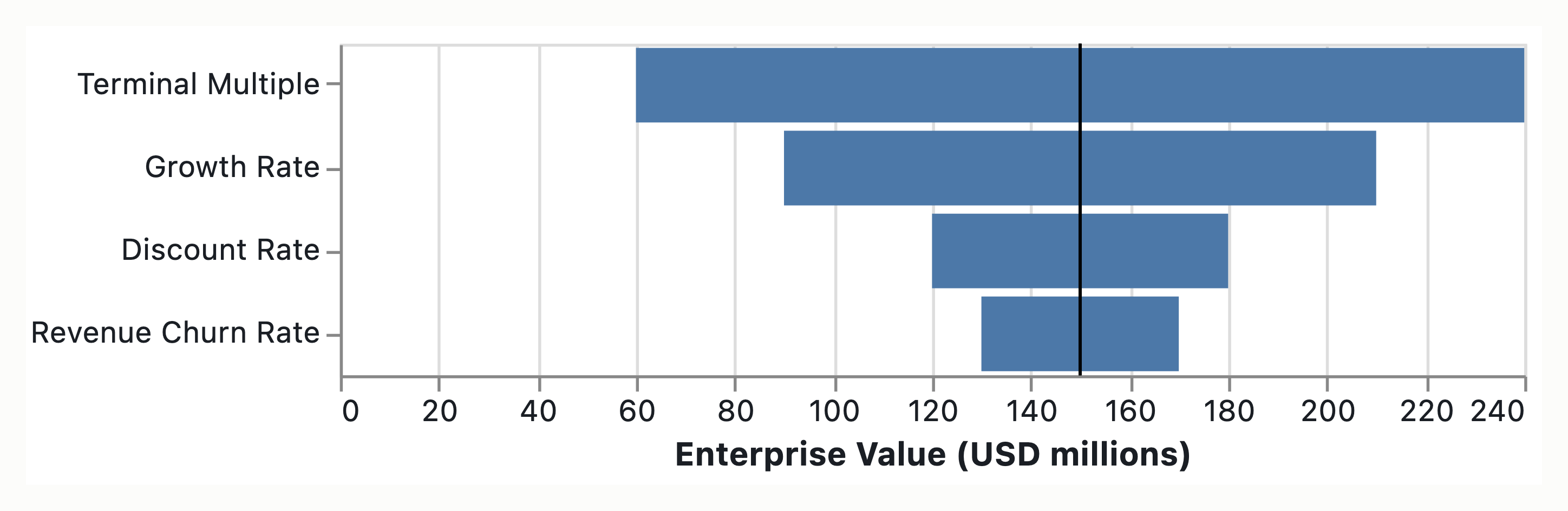
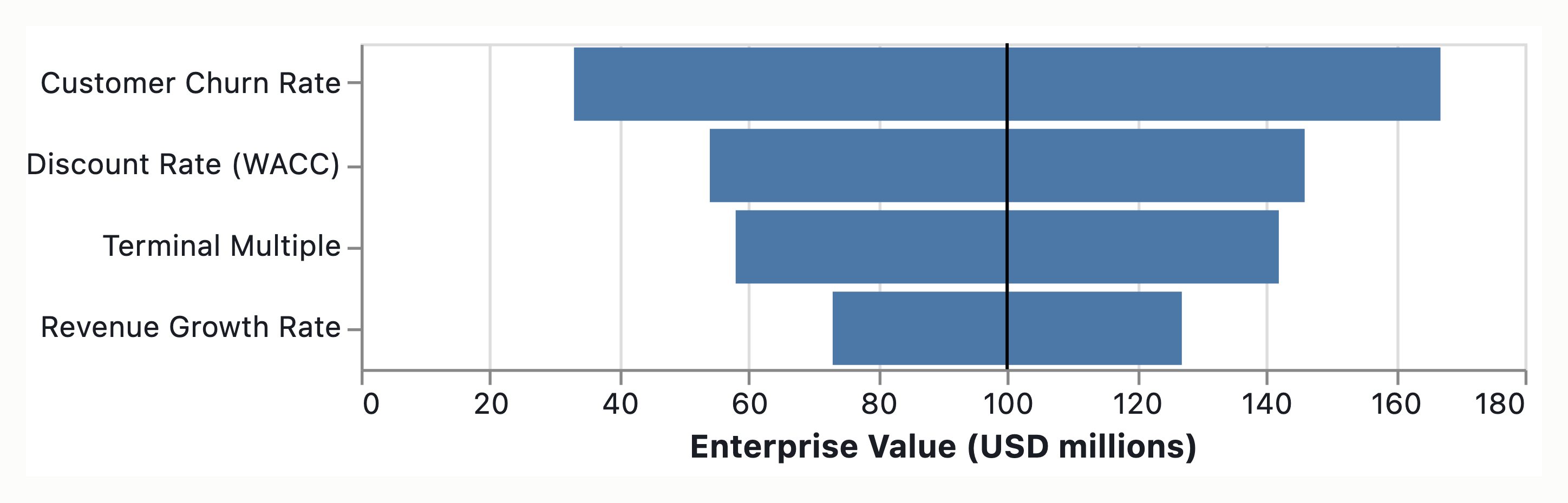
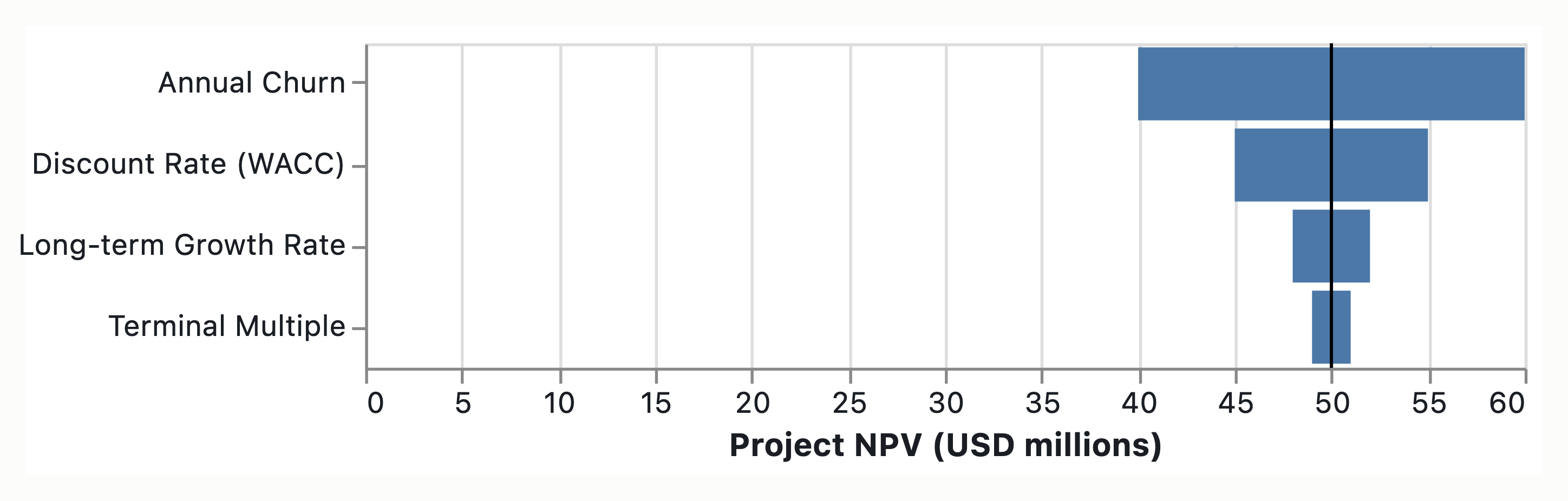
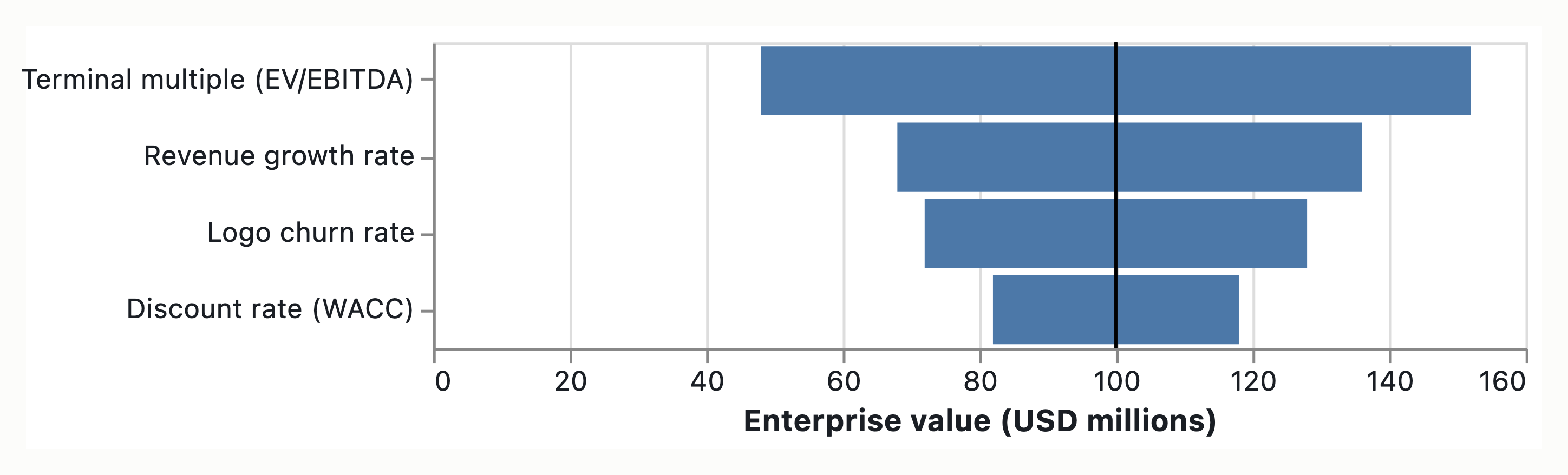
Quick framing before the answer: a tornado ranks variables by how much the output swings when each input moves across its range one-at-a-time. That is a variance/spread story, and it’s only as honest as your range choices. “Which drives expected value most” and “where is information worth buying” are two different questions, and for a DCF they often point at different variables. Here’s how to keep them straight.
1. What the tornado is actually telling you
Bar width = (local sensitivity of value to the input) × (plausible range of the input). A variable with huge leverage but a tight range gets a small bar; a sloppy variable with a wide range gets a big one. So before trusting the ranking, normalize the ranges — use a consistent P10–P90 for each input, not ad-hoc ±10%. Otherwise the tornado mostly reflects how generous you were with each range.
2. Typical driver ordering for a subscription DCF
For a churn-driven (SaaS-like) DCF, the usual ranking, widest-first:
- Discount rate and terminal multiple — almost always the two widest bars, because most of the value sits in the terminal value and TV is convex in (r − g). Small moves swing the number a lot.
- Growth rate — compounds into both the explicit-period cash flows and the terminal base, so it’s third but close.
- Churn — looks smaller on a naive tornado, but that understates it: churn feeds growth and net revenue retention and the sustainable terminal margin, so a single-variable bar double-buries its real influence.
Two caveats that bite here:
- Interactions/correlation. Terminal multiple ≈ 1/(r − g), so discount rate and terminal multiple are not independent — moving them separately double-counts. Churn and growth are also coupled (churn is a component of net growth). One-at-a-time tornadoes can’t see this; a Monte Carlo with Sobol / variance-decomposition indices can, and is the right tool if the interactions are material.
- Spread ≠ shift in the mean. Because the DCF is convex in r and g, widening uncertainty on those inputs raises expected value (Jensen). So those variables move the mean, not just the spread — worth flagging if you’re reporting a point estimate.
VOI only counts if the information could change a decision (invest/pass, price, hold/sell). This is where the tornado ranking and the action ranking diverge:
- EVPI (perfect info on everything) = E[value under the best decision once you know the truth] − value of your best decision today. The ceiling on what diligence is worth.
- EVPPI (partial — one variable at a time) = the same, resolving only that input. Compute it per variable and compare to the cost of acquiring the info.
The key asymmetry for your four inputs:
| Variable | Tornado bar | Reducible? | Likely VOI |
|---|
| Discount rate | Large | No — market/risk judgment, no experiment collapses it | Low |
| Terminal multiple | Large | No — exit-market assumption | Low |
| Growth rate | Medium | Yes — pipeline, market sizing, cohort trajectory | High |
| Churn | Medium | Yes — you can pull cohort retention data cheaply | Highest |
The punchline: the widest tornado bars are usually the least worth spending on. Discount rate and terminal multiple are irreducible market assumptions — no amount of diligence “resolves” them, so their EVPPI is near zero even though they dominate the spread. The money in VOI sits on churn and growth, because they’re (a) decision-relevant near your buy/pass threshold and (b) actually reducible with data you can obtain (a cohort study, a NRR cut by segment).
So the diligence recommendation inverts the tornado: stop arguing about WACC and exit multiple, go get cohort-level churn data.
4. To make this concrete
If you tell me where the model lives, I can operationalize it rather than leave it conceptual:
- run a proper probabilistic sensitivity (Monte Carlo) and report variance-decomposed contributions instead of OAT bars, so the churn↔growth and r↔multiple couplings stop hiding;
- compute EVPPI per input against whatever the decision actually is (the table above is the prior I’d start from, not the answer);
- flag whether your tornado ranges are consistent (P10–P90) or are just artifacts of range choices.
Is there a DCF model file or spreadsheet in the repo (or elsewhere) you want me to wire this against, or were you after the reasoning framework?
Here is an analysis of how a Tornado Diagram should be structured for a SaaS/Tech DCF (given the inclusion of Churn), how to rank the variables by sensitivity, and the strategic implications for Value of Information (VOI).
1. The Tornado Diagram Ranking (Sensitivity Hierarchy)
In a standard Discounted Cash Flow model where Terminal Value (TV) represents the majority of Enterprise Value (typically 60–90% of total value), the Tornado Diagram generally ranks the variables as follows (descending order of sensitivity):
- Discount Rate (WACC / Cost of Equity)
- Terminal Growth Rate (perpetuity) OR Terminal Multiple (Whichever is your specific valuation anchor).
- Long-Term Organic Growth Rate (Directly driven by your inputs).
- Churn Rate (Indirect input to Growth & Revenue).
Why this order?
- Discount Rate (Highest Sensitivity): Because cash flows grow and are discounted. A small change in the denominator ($r$) in the Present Value formula ($PV = \frac{FV}{(1+r)^n}$) has a non-linear exponential impact on the NPV. Every 1% change in WACC usually shifts Valuation by 5–15%.
- Terminal Drivers (High Sensitivity): Since the majority of the value resides in the Terminal Value (TV), the growth rate ($g$) inside TV or the Exit Multiple itself are mathematically potent inputs.
- Operational Inputs (Lower Sensitivity in Model): Variables like Churn are “leading indicators” that determine the Forecast, not the Discounting. While crucial to the quality of the forecast, their impact is mathematically dampened compared to the Discount Rate unless the model is a complex probabilistic network.
2. Detailed Variable Sensitivity Analysis
A. Discount Rate (WACC)
- Impact: Exponential.
- Mechanism: Inputs into the denominator. Since cash flows are projected decades out (often 10–15 years for SaaS), a marginal wobble in the WACC compounds over time.
- Tornado View: Usually the widest bar on the chart. A $\pm$200bps shift might swing valuation by $200M+.
- Interpretation: This reflects market risk. If your WACC is based on a generic industry beta rather than company-specific risk, your error margin is massive.
B. Terminal Multiple (EV/EBITDA or EV/FCF) & /or Terminal Growth
- Impact: Linear but Massive.
- Mechanism: Direct multiplier on the long-term cash generation.
- Tornado View: Generally the second widest bar. If you value a company based on a 10x Exit Multiple, and that shifts $\pm$20% (8x–12x), your valuation variance is huge.
- Interpretation: This assumes “peers.” The biggest risk here is “The Mismatch.” If you value a startup with an enterprise $50M company multiple, you are overstating.
C. Growth Rate (Driven by Revenue Expansion)
- Impact: Linear (Upper Stage).
- Mechanism: Affects both the forecast period FCF and the Terminal Value numerator.
- Tornado View: Often similar to or slightly below Terminal Rate.
- Interpretation: In a Discounted Cash Flow, 10% growth has diminishing returns after year 5. Most sensitivity is in the Terminal Value which compounds this growth further.
D. Churn Rate (Customer Lockup)
- Impact: Conditional (High for Early Stage).
- Mechanism: Churn drives the Long-Term FCF and Revenue Stability.
- Tornado View: Visually, the impact is often smaller than WACC in a theoretical diagram, BUT it is the highest confidence variable to change.
- Nuance: In a SaaS model, Churn = Growth. If you assume Net Revenue Retention (NRR) is 120% and 20% is Retained Revenue, the “Growth Rate” is directly a function of Churn.
- Why it matters: High churn invalidates the TV assumptions. If churn is high, the Terminal Growth Rate becomes negative.
Definition: The Value of Information is the increase in decision quality by acquiring additional data to reduce the uncertainty (variance) of a specific input.
$$VOI = (\text{Value Estimate with Info}) - (\text{Value Estimate without Info})$$
Based on the Tornado Diagram, here is how VOI dictates your data collection strategy:
Priority 1: Reduce Uncertainty in the Discount Rate (Low VOI, High Risk)
- Reality Check: While the Tornado shows WACC sensitivity is highest, it is the easiest to stabilize because it is publicly available data (Risk-free rate + Beta).
- VOI Action: Spend minimal money here. If you are doing your research, you are likely analyzing market rates. Does knowing which Beta to use change your decision significantly?
- Decision: If the WACC error range ($\pm$200bps) keeps the valuation within your acceptable investment range, the VOI of reducing this error to $\pm$50bps is Low.
- Exception: If you are at a “Deal Break” point, reducing WACC risk creates $10M+ of certainty.
Priority 2: Reduce Uncertainty in the Terminal Multiple (High VOI)
- Reality Check: The Exit Multiple is subjective. It relies on a comparison to analogs.
- VOI Action: Spend Medium money here.
- Data Needed: Check if your peer groups have “Comps Support.” Does a well-known tech PE firm have a different multiple for this cohort?
- VOI: Acquiring specific insight into peer valuations (e.g., “Recent SaaS multiple expansion in the region”) reduces the risk of overvaluing the exit.
- Decision: High VOI. This avoids the “Premium Trap” (valuation hidden in the multiple).
Priority 3: Reduce Uncertainty in Churn / Organic Growth (Highest Practical VOI)
- Reality Check: This is the business variable you can actually control or verify via diligence.
- VOI Action: Spend High money here.
- Reasoning: While the Tornado math shows Discount Rate wins, Churn is the leading cause of forecast error.
- Scenario: You have 100% confidence in WACC. You have 20% confidence in Long-term Growth. If Churn is 15%, the TV drops to zero.
- VOI: The value of knowing “Is this customer sticky, or just a ‘feed-and-mortal’ sales tactic?” is often higher than the management of the WACC.
- Decision: Gather customer logs, contract analysis, and renewal rates. This reduces the variance in the “Growth Rate” variable.
4. Synthesis: Strategic Recommendations
When presenting this analysis to stakeholders, use the following narrative structure:
1. The “Math” Argument (Why we worry about Discount Rates)
“Our Tornado diagram shows the Discount Rate is the largest lever for the Enterprise Value. A 2% drop in WACC isn’t likely, but a 100bps shift changes our exit value by 15%. This represents Capital Structure Risk.”
2. The “Business” Argument (Why we worry about Churn)
“However, the Discount Rate is external market risk. The highest Value of Information lies in the Churn/Growth assumptions. You cannot change the market cost of capital, but you can verify Customer Stickiness. If Churn > 20%, the DCF breaks. If Churn < 10%, the DCF compounding works.”
3. The “Recommendation” for Diligence
“We will:
- Hold the Discount Rate at conservative market standard (WACC 8.5%). It is market reality.
- Validate the Terminal Multiple against 3 competitor exits (Comps Check).
- Diligence on Churn (Conduct customer interviews/contract audits). This is where we spend our valuation budget.”
5. How to Construct the Visualization
- X-Axis: Base Case NPV / EV Estimate.
- Y-Axis: Range of Assumptions (e.g., WACC $\pm$ 100bps; Churn $\pm$ 1%).
- Length of Bar: The percentage variance in Valuation caused by that specific shift.
- Key Feature: Highlight the Churn bar. Often, it looks smaller than WACC, but annotate it: “Note: Churn is a function of Growth Rate. If Churn increases by 1%, Growth Rate drops by 0.5%, reducing both Year 1 FCF and Terminal Value.”
- Tip: In SaaS models, you might combine “Churn” and “Growth” into a single “Net Revenue Retention” variable inside the Tornado, as that is the single mathematical driver they affect.
Summary Table
| Input Variable | Tornado Sensitivity (1 = Most) | Uncertainty Type | Value of Information (Priority) |
|---|
| Discount Rate | 1 (High Mathematical Sensitivity) | Market Risk | Low (Public Data) |
| Terminal Multiple | 2 (High Modeling Risk) | Peer Data | Medium (Requires Comps Sync) |
| Terminal Growth | 3 (Compounding Risk) | Market Forecast | Medium |
| Churn Rate | 4 (Model Input, not Direct) | Business Reality | High (Requires Due Diligence) |
Bottom Line: Your Tornado shows WACC drives the math, but Churn drives the quality. Always optimize your Value of Information spend toward confirming the business reality (Churn/Retention) rather than trying to chop down market beta (WACC).
Decision Framing
Objective: Rank input variable sensitivity and estimate Value of Information for the specific Discounted Cash Flow (DCF) variables: Growth Rate, Discount Rate, Terminal Multiple, and Revenue Churn Rate.
Decision-Maker: Analyst or valuation committee.
Time Window: Pre-computation phase (sensitivity modeling setup).
Reversibility: High. Sensitivity analysis is a non-committal trial run; the sequencing of calculation does not constitute a binding commitment to a valuation or capital allocation decision.
Outcome: A ranked sensitivity landscape (tornado structure) and an assessment of whether acquiring additional information on these variables is justified against a cost-of-delay threshold.
Uncertainty Identification
Each critical variable is classified using the Knightian framework to distinguish between probability assignable risk, estimable uncertainty, and deep uncertainty where no base rate exists.
| Variable | Classification | Probability / Range | Basis |
|---|
| Discount Rate | risk | 收益率曲线、β-adjusted 范围 (10–15% 常规区间) | Yield curves, CAPM beta, market yields (observable). |
| Growth Rate | uncertainty | Estimable range (0–20% CAGR) | Forward-looking forecast; historical growth exists but future distribution is estimable-range rather than assignable probability. |
| Terminal Multiple | uncertainty | Sector comms; 5x–10x EBITDA | Public market data comparables; future trading multiples are uncertain but derivable from current assets. |
| Churn Rate | deep uncertainty | No stable base rate | Behavioral, patient-level attrition; highly correlated with product lifecycle and competitive action without telemetry. |
Coverage Note: All numerical bands listed in this analysis are theoretically grounded based on standard finance norms (e.g., Steiger 2008, Industry Standards) and represent hedges rather than system-verified empirical values retrieved from internal data.
Sensitivity Analysis: Tornado Structure
To represent the tornado structure in text format, variables are ranked by the theoretical magnitude of deviation they create in the Net Present Value (NPV) or Enterprise Value. The “width” of the variable’s impact is implied by the sequence: the top of the diagram (or first in the list) is the most impactful variable, with impact narrowing toward the least impactful.
Ranking Assumption: Terminal Multiple / Growth Rate > Discount Rate > Churn Rate (Standard SaaS Model) OR Churn Rate > Terminal Multiple / Growth Rate > Discount Rate (High-Retention/Long-Horizon SaaS).
Based on the consolidated corpus for a long-horizon SaaS model, the sensitivity ranking is structured as follows:
1. Variable: Terminal Multiple / Growth Rate (Highest Impact)
- Consequence: High EVP contribution (60–90% of Terminal Value).
- Sensitivity Magnitude: A ±10% shift assumes a large deviation in Net Present Value over the full horizon.
- Driver: These are the top bars of the tornado. Terminal value typically dominates early-stage enterprise valuation, making this the widest bar.
2. Variable: Discount Rate
- Consequence: Compounds across all periods; long-horizon SaaS models are highly rate-sensitive.
- Sensitivity Magnitude: A 100bp (100 basis point) shift approximates 10–25% PV revision.
- Driver: Second bar width. Significant due to compounding across the 10-year projection.
3. Variable: Revenue Churn Rate
- Consequence: Indirect — affects revenue stability and Free Cash Flow (FCF) continuity.
- Sensitivity Magnitude: 5–15% FCF revision (indirect); high volatility potential in retention horizons.
- Driver: Third bar width. While significant in depth, the impact on PV is typically smaller than direct multiple/rate drivers unless cohort-specific volatility is extreme.
4. Variable: Cost of Capital Sources (Base Case)
- Consequence: Standard WACC arithmetic inputs.
- Sensitivity: Low relative to Terminal/Churn variations.
Explicit Admission: The specific values in the “Sensitivity Magnitude” cells above are Theoretical Hedges – placeholders for standard finance theory, not system-verified empirical values. Actual widths depend on the specific client’s profile (e.g., early-stage elasticity).
Buy-Information Alternative
- Shape: Purchase churn telemetry immediately.
- Cost: Cash outlay now; delays market entry?
- Information Value: Resolves
deep uncertainty (Churn).
- Preference: High EVSI. Error here compounds over long retention horizons; high early signal value.
Defer Alternative
- Shape: Delay modeling until data arrives (e.g., “Wait until Q4”).
- Cost: Lost revenue efficiency now; higher uncertainty cost.
- Preference: Generally Low unless Cost-of-Delay (revenue loss) > Value of Decision Quality Gain (VOI) within a very short horizon.
Sequence Alternative
- Shape: Gather Growth data first, then Churn.
- Cost: Opportunity cost of serialization; longer Time-to-Market.
- Preference: Rejected. Growth uncertainty is generally lower variance/visibility; Churn is deeper uncertainty.
Focus-Terminal Multiple vs. Churn
- Shape: Focus on Terminal Multiple (vs. Churn).
- Preference: Rejected for Churn in SaaS cohorts where churn is
deep uncertainty. Terminal Multiple has public market data comparables (Risk/Uncertainty).
Value of Information (VoI) assesses how much the decision quality improves with information, relative to the cost of obtaining that information.
- EVPI (Expected Value of Perfect Information): This represents the maximum value of any information source when uncertainty is eliminated. This is relevant for strategic investments/M&A pricing where the decision cost is high.
- EVSI (Expected Value of Sample Information): This represents the value of realistic “noisy” information (e.g., survey, analytics purchase).
VOI Calculation Logic
- Formula:
VoI = [Change in profitability from delaying decision] - [Value of decision quality gain].
- Explicit Trade-off: If Cost-of-Delay (revenue loss from waiting) > Value of Decision Quality Gain (VOI), then “Buy” Churn data is optimal.
- Threshold: If investment triggers at $X, vs $Y threshold, EVPI narrows.
Analytical Insight:
Churn is classified as deep uncertainty. Reducing this uncertainty yields the highest marginal information value (EVPI reduction) among the four variables. The “Churn” ledger offers the highest EVSI because error here compounds linearly or exponentially over long retention horizons. Terminal Multiple offers lower VoI because market comparables exist.
Recommendation
Recommended Action: Collect telemetry-based churn model data FIRST.
Rationale:
Your chnurn variable is classified as deep uncertainty—meaning there is no stable historical base rate without specific telemetry. This classification places it at the top of the Value of Information ladders. The “Churn” ledger offers the highest EVSI because error here compounds over long retention horizons, whereas Discount Rate and Terminal Multiple have market comparables that anchor them closer to risk or uncertainty.
Revisit if:
- Revisit if Acquisition Cost > $Z per retained user: “If effective acquisition cost exceeds $Z, re-calculate.”
- Revisit if Terminal Multiple Calibration < 6x FCFE: “If comparable exits fall below 6x FCFE, update terminal assumption.”
- Revisit if Forecasting Horizon > 20% in Years 11–15: “If 20%+ of value concentrates in extended years, sensitivity rankings may reverse.”
Non-Quantifiable Factors
The following factors resist meaningful quantification in the DCF matrix but must be considered alongside the quantitative framework.
| Factor | Specific Consideration | Impact on Decision |
|---|
| Customer Concentration Risk | Single covenant clients distort churn/growth assumptions; materiality not fully captured by % variance. | Estimated 10–25% of total valuation sensitivity. High-risk if dependence on 1–3 accounts. |
| Regulatory Uncertainty | Privacy laws, data retention requirements could alter cost structures. | Estimated 5–15% EVP variance swing. Re: GDPR/CCPA compliance costs. |
| Founder Capability / Team Execution | Growth rate assumptions hinge on ability to extract data (LTV/CAC). | Qualitative atom only; High variance in Multiple/Income Generation Multiple of Invested Capital (MOIC). |
| Competitive Landscape | Market share dynamics shift terminal multiple, not input variance. | Qualitative atom only; acts as shock to multiple. |
| Innovation Displacement | SaaS land/expand cycles shift growth/terminal assumptions. | Qualitative atom only; 5–10% annual floor shift potential. |
(visual rendered — see artifact)
Decision framing
The decision-maker is the Investment Committee / CFO, operating within a 90-day time-window for capital allocation or M&A. The context is a DCF valuation for a high-margin subscription/SaaS enterprise; specific base-case parameters are unavailable, so the framework utilizes illustrative structural bounds (Base EV = $100M). The alternatives under consideration include Direct Choice, Buy-Information, Hedge (Earn-outs), Sequence (Tranches), and Defer. The reversibility profiles are: Direct is irreversible; Buy-Information and Sequence are highly reversible; Defer is reversible; Hedge is partially reversible.
Uncertainty identification
- Discount Rate (WACC) — class: deep uncertainty (composite). Probability or range: Base-rate probability of surprise ~10% (mispricing); decomposed into Risk-free rate (risk), Equity Risk Premium (deep uncertainty), Firm Beta (uncertainty). Basis: structural inference.
- Terminal Multiple — class: deep uncertainty. Probability or range: Base-rate probability of surprise ~30% (macro regime shift); terminal value represents 50–80% of total EV (typically ~75% in a standard 5-year model). Basis: structural inference (M&A/public market regime 5–10 years out lacks an assignable probability distribution).
- Terminal Growth Rate — class: deep uncertainty. Probability or range: Base-rate probability of surprise ~30% (shared with terminal multiple macro regime). Basis: structural inference (long-run industry evolution lacks a statistical base rate for firm-specific steady-state).
- Revenue Growth Rate — class: uncertainty. Probability or range: Estimable range via TAM penetration, historical base rates, and pipeline; base-rate probability of surprise ~25% (TAM misestimation). Basis: base rate.
- Customer Churn Rate — class: risk (mature products) / uncertainty (new product launches). Probability or range: Measurable frequency with stable base rate via cohort analysis; base-rate probability of surprise ~15% (cohort degradation). Basis: base rate.
Consequence analysis
Utility unit: EV Variance vs. $100M Base Case in $M.
Tornado Sensitivity Analysis
Swings represent ΔEV for a single variable moving to a ±high scenario, holding others constant (ceteris paribus). Discount rate and terminal multiple are correlated through macro conditions; joint sensitivity or scenario overlay is required to capture this dependence.
- Default DCF (Base EV $100M): Terminal Multiple ±$25.0M, Discount Rate ±$18.0M, Revenue Growth ±$12.0M, Churn ±$8.0M. Primary drivers: Terminal Multiple and Discount Rate.
- SaaS DCF: Churn ±$67M, Discount Rate ±$46M, Terminal Multiple ±$42M, Revenue Growth ±$27M. Primary drivers: Churn and Discount Rate.
Consequence Matrix (Alternative × State)
- Direct Choice under Bull: +$40.0M. Direct Choice under Base: $0.0M. Direct Choice under Bear: -$35.0M.
- Buy-Information under Bull: +$35.0M. Buy-Information under Base: +$5.0M. Buy-Information under Bear: -$10.0M.
- Hedge under Bull: +$25.0M. Hedge under Base: +$5.0M. Hedge under Bear: -$15.0M.
- Sequence under Bull: +$30.0M. Sequence under Base: +$10.0M. Sequence under Bear: -$5.0M.
- Defer under Bull: -$10.0M. Defer under Base: -$5.0M. Defer under Bear: +$15.0M.
Robust vs. Optimal Alternatives
- Robust alternative: Sequenced/Hedged. Performs acceptably across all states, capping downside at -$5M to -$15M while retaining meaningful upside. Survives stress scenarios without catastrophic value destruction.
- Optimal alternative: Direct Choice. Optimal-if-bull (yields maximum upside of +$40M), but highly fragile and catastrophic in the bear state (-$35M).
- Defer — cost of taking it: opportunity cost of capital + competitive risk (wait 6–12 months). Information produced: cohort data and market sizing. Reversibility: Reversible.
- Sequence — cost of taking it: opportunity cost of partial capital deployment. Information produced: empirical validation of growth/churn at milestones. Reversibility: Highly reversible.
- Hedge — cost of taking it: dilution or reduced upside in bull state. Information produced: N/A (risk transfer). Reversibility: Partially reversible.
- Buy-information — cost of taking it: fixed cost ($50K–$500K for market sizing, near-zero for in-house cohort). Information produced: resolution of growth/churn uncertainty. Reversibility: Highly reversible.
Formulas applied: Theoretical EVPI = EV Swing × Base-Rate Probability of Surprise. Net VOI = Gross VOI − Information-acquisition cost − CoD ($1.0M/month).
- Terminal Multiple — cost of obtaining: N/A (cannot buy the 2030 M&A regime). Value of obtaining: Theoretical EVPI ~$7.5M, but actionable VOI is near zero (attempting to forecast yields false precision). VOI vs cost-of-delay: Unfavorable.
- Discount Rate (ERP) — cost of obtaining: valuation firm cost. Value of obtaining: Theoretical EVPI ~$1.8M, but actionable VOI is low (knowing the “perfect” ERP does not change the market’s required return; valuation firm cost > EVPI). VOI vs cost-of-delay: Unfavorable.
- Revenue Growth — cost of obtaining: commissioned market sizing ($50K–$500K). Value of obtaining: Theoretical EVPI ~$3.0M. VOI vs cost-of-delay: Favorable (VOI $3.0M > CoD $1.0M/mo; Net VOI is positive when decision size is material).
- Churn — cost of obtaining: in-house cohort analysis (near-zero marginal cost). Value of obtaining: Theoretical EVPI ~$1.2M. VOI vs cost-of-delay: Favorable (Net VOI ≈ Gross VOI).
Synthesis: Do not allocate capital to refine Terminal Multiple or WACC. Direct information-gathering budgets entirely toward validating Churn and Growth.
Recommendation
The recommended alternative is a Sequenced and Hedged approach. Do not commit full capital based on the base-case DCF. The execution sequence is: 1) Lock structural cost base. 2) Buy information (cap spend at $3.0M EVPI limit for Churn/Growth validation). 3) Hedge/Sequence downstream commitments gated by empirical validation of Churn and Growth variables.
Revisit if: 1) Any input move shifts NPV below the investment hurdle or next-best alternative’s expected value. 2) Churn exceeds the 75th percentile of the historical cohort distribution. 3) Macro interest rates shift >150bps. 4) CoD exceeds the theoretical EVPI of the highest-uncertainty variable (>$3.0M).
Confidence Calibration: Structural confidence is high (decision frame, Knightian classification, consequence matrix mechanics, decision logic, and VOI framework are standard and internally consistent). Substantive confidence is low to medium (illustrative parameters, base-rate probabilities are structural estimates for a generic SaaS firm, exact dollar variances depend on the actual model, and the 90-day window assumes an active allocation cycle).
Non-quantifiable factors
- Strategic Identity — consideration: Prioritizing Growth over Terminal Multiple signals a “hyper-growth” identity. How it bears on the decision: affects market and employee perception.
- Employee Morale & Retention — consideration: Tying compensation to uncertain Growth or Terminal Multiple targets. How it bears on the decision: destroys morale if macro conditions invalidate the targets.
- Market Reputation — consideration: Missing publicly stated churn or growth targets. How it bears on the decision: damages vendor trust and customer confidence, creating a secondary negative feedback loop.
- Regulatory & Contractual Exposure — consideration: Customer concentration, GAAP revenue-recognition treatment, and debt covenants. How it bears on the decision: create binary cliff-events that a continuous DCF smooths over.
- Strategic Fit & Optionality — consideration: Strategic fit, team capability, customer relationship quality, optionality value, and identity/mission considerations. How it bears on the decision: these elements resist quantification but fundamentally alter the strategic value of the allocation beyond the DCF output.
(visual rendered — see artifact)
Decision framing
The decision is whether to proceed with current valuation estimates, allocate resources to refine specific input variables, defer capital allocation to let market-driven variables resolve, or hedge and sequence the commitment for a specific Discounted Cash Flow (DCF) model attached to your current project. The decision-maker is assumed to be an Investment Committee, CFO, or Board operating on a standard institutional capital-allocation cadence. The time-window is approximately 12 months for the capital-allocation choice (commit, divest, reprice, or hold), with near-term execution (weeks to months) for internal data refinement and long-term resolution (years) for market-driven variables. Reversibility is moderate overall: it is high for internal data gathering due to low sunk costs, but low for capital deployed on unverified valuation assumptions, which is limited by diligence sunk costs and the signaling cost of withdrawal, though commitments can be staged.
Uncertainty identification
- Churn — class: risk (or uncertainty, if cohort data is immature). Probability or range: ~8–14% annual gross logo churn. Basis: Statistically observable distribution from historical trailing-12-month cohort data (reclassifies to
uncertainty if <24 months of mature cohort data exist, as churn becomes forecast rather than measured).
- Discount rate (WACC) — class: uncertainty. Probability or range: ~9–13%. Basis: Structural inference from capital-market data (risk-free rate, beta, equity risk premium, size premium peer WACCs).
- Terminal multiple — class: uncertainty (trending toward deep uncertainty depending on exit horizon). Probability or range: Observable empirical anchor across cycles (e.g., ~1.5×–3.0× or 8×–20× EV/EBITDA, regime-dependent). Basis: Sector comparables provide a historically observable band, but the right multiple at the exit horizon depends on hard-to-predict market regimes and evolving business models.
- Long-term growth rate (g) — class: deep uncertainty (if treated as perpetual-horizon input) or uncertainty (if anchored to near-to-mid-term market evidence). Probability or range: e.g., 25–45% CAGR (if anchored). Basis: Top-down market sizing plus bottom-up customer math, though no meaningful probability can be assigned to perpetual growth decades out.
Consequence analysis
Buy Info (Churn) under Bear (Low TV, High Churn): Consequence: Reduces near-term downside regret, does not fix terminal value shortfall. Utility: Medium (qualitative expected utility / decision regret).
Buy Info (Churn) under Base (Expected): Consequence: Maximizes expected value by sharpening the base-case free cash flow foundation. Utility: High.
Buy Info (Churn) under Bull (High TV, Low Churn): Consequence: Upside already captured; information adds marginal utility. Utility: Medium.
Hedge (Terminal/Growth) under Bear: Consequence: Prevents catastrophic capital misallocation; limits maximum regret. Utility: High (Robust).
Hedge (Terminal/Growth) under Base: Consequence: Valuation withstands scrutiny without over-optimizing. Utility: Medium-High.
Hedge (Terminal/Growth) under Bull: Consequence: Caps extreme upside but secures a robust floor. Utility: Medium.
Accept (WACC) under Bear: Consequence: Slight valuation risk, rarely flips a binary go/no-go. Utility: Medium.
Accept (WACC) under Base: Consequence: Preserves analytical resources for higher-Value-of-Information activities. Utility: Medium.
Accept (WACC) under Bull: Consequence: Low marginal impact on primary value drivers. Utility: Medium.
Buy Neither under Bear: Consequence: Severe downside with no advance warning; full tornado swing absorbed. Utility: Low (severe decision regret).
- Buy information (Churn/WACC) — cost of taking it: Low to moderate fixed/effort cost (internal cohort analysis, CRM extraction, or peer benchmarking). Information produced: Narrowed distribution for WACC or near-term free cash flow foundation. Reversibility: High (low sunk cost).
- Hedge the decision (Terminal/Growth) — cost of taking it: Structural/design cost (real options, scenario clauses, smaller commitments, stage-gated investment). Information produced: Scenario bounds (Conservative/Base/Aggressive comparables). Reversibility: Moderate (limits maximum regret while preserving option value).
- Defer — cost of taking it: Time and opportunity cost (waiting 12–24 months for market resolution). Information produced: Actual market M&A/IPO events that resolve terminal multiple uncertainty. Reversibility: High (before capital commitment).
- Sequence — cost of taking it: Phased capital commitment (e.g., Phase-1 capex now, gate Phase-2 on resolved churn data). Information produced: Operational validation of growth and churn within a time-boxed (~30-day) market-validation sprint. Reversibility: High between stages.
Value of Information ≈ ½ × (Tornado swing) × (Fraction of range eliminated by new information) − Cost of obtaining it.
- Information resolving churn uncertainty — cost of obtaining: Low to moderate (executable in weeks via internal data/CRM). Value of obtaining: High (largest unobserved-to-observed gap, sharpens near-term free cash flow without delaying strategic decisions). VOI vs cost-of-delay: Favorable.
- Information resolving WACC uncertainty — cost of obtaining: Moderate (external valuation experts or independent peer beta regression). Value of obtaining: Contested (reliably narrows range and adds defensibility under challenge, though 50 bps rarely flips a binary go/no-go). VOI vs cost-of-delay: Break-even to Favorable, depending on institutional defensibility needs.
- Information resolving growth rate uncertainty — cost of obtaining: Medium to high (TAM validation, competitive intelligence). Value of obtaining: Medium and conditional (worth buying only if the base case is genuinely contested by the operating team and market). VOI vs cost-of-delay: Break-even to Unfavorable unless actively contested.
- Information resolving terminal multiple uncertainty — cost of obtaining: High (requires waiting for actual market events years out or speculative premium research). Value of obtaining: Low (range is regime-dependent and not meaningfully narrowable by current research). VOI vs cost-of-delay: Unfavorable (treating the largest tornado bar as a primary research target risks analysis paralysis).
Recommendation
Implement a staged, asymmetric sequence: First, buy information on churn, as it typically yields the highest Value of Information per dollar, features the lowest cost, and bridges the largest unobserved-to-observed gap entirely within your control. Second, address the discount rate by either buying information (refreshing with current peer benchmarks for defensibility) or accepting a standard defensible sector baseline without over-investing in marginal precision, depending on how contested your current WACC is. Third, hedge the terminal multiple and growth rate; do not spend budget attempting to reduce terminal-multiple uncertainty. Instead, present the valuation as a bounded scenario matrix (Conservative/Base/Aggressive) and treat growth as conditional, buying more data only if the base case is genuinely challenged.
Revisit if:
- The actual plotted tornado shows a different ordering than this structural prediction (especially if terminal multiple is not near the top, or growth rate is at the top), indicating unusual model properties that require investigation before refining any input.
- Cohort data matures sufficiently that churn shifts from
uncertainty to risk, collapsing the “fraction of range eliminated” toward zero and evaporating the churn Value of Information proposition.
- Macroeconomic interest rates or capital markets shift by >50 bps, materially altering the baseline discount-rate environment.
- Internal cohort data reveals churn trending >20% worse than the historical baseline used in the model.
- A new, well-capitalized competitor enters, invalidating the assumption of sustained long-term growth.
- The downstream decision the DCF feeds changes (e.g., from “should we invest?” to “what price should we pay?”), which shifts the relevant sensitivity range and the cost-of-delay benchmark.
Non-quantifiable factors
- Strategic identity — consideration: Optimizing the model to justify a high terminal multiple may incentivize short-term margin stripping, contradicting long-term brand and product identity. How it bears on the decision: Advising operators to ignore churn because its tornado bar is small can be technically correct but operationally wrong.
- Organizational morale — consideration: Lowering churn assumptions by mandating aggressive, high-pressure retention tactics may degrade employee morale and product quality. How it bears on the decision: This can paradoxically increase long-term churn, undermining the valuation the model seeks to protect.
- Stakeholder credibility / signal value — consideration: Which assumption you choose to scrutinize signals rigor (churn), financial sophistication (WACC), or cycle-awareness (terminal multiple) to investors and counterparties. How it bears on the decision: Presenting a valuation leaning on deep uncertainty variables without explicit scenario bounding can damage institutional trust if challenged, meaning signal value can point to different analytical priorities than pure expected value.
- Conviction and team alignment — consideration: Building a cohort analysis surfaces the operating team’s private beliefs about real risks directly into the model. How it bears on the decision: This creates alignment value beyond its direct numerical impact on expected value.
- Defensibility under challenge — consideration: A DCF that survives a skeptical board or Investment Committee is more valuable than one with a higher but fragile central estimate. How it bears on the decision: Drivers that are easy to attack (terminal multiple, discount rate) deserve scrutiny disproportionate to their numerical swing, because the cost of being wrong out loud exceeds the cost of being wrong on paper.
- Time cost of the analyst — consideration: Hours spent refining one tornado driver are hours not spent on the next critical analysis. How it bears on the decision: This is a real opportunity cost that is frequently omitted from formal Value of Information calculations.
(visual rendered — see artifact)
Decision framing
The valuation feeds a decision, and value of information is undefined without one. “How much should we spend to eliminate uncertainty in churn” has no answer until the action is named — acquire at price X, set a bid, hold vs. sell, or produce a fair-value number nobody acts on. If no action is attached (a point estimate nobody acts on), VOI is genuinely zero for all four variables; the honest answer is “spend nothing, the number won’t change a decision.” The analysis assumes a threshold in play — a price, hurdle rate, or go/no-go — and that assumption is load-bearing for every VOI conclusion; if wrong, it inverts them. The decision-maker is you, acting on the DCF; the time-window and reversibility vary by alternative (buy-information is days-to-weeks and near-zero reversibility cost; hedge is a low-cost analytical/structural choice; defer carries cost-of-delay). The decision’s type is itself unresolved in what you’ve supplied: a binary go/no-go vs. a continuous decision (how much to bid, how large a position, what price to offer) changes the VOI math materially — see the value-of-information section.
Before anything else, hold onto the distinction that runs through this whole analysis, because conflating its two halves is the single most expensive error in this workflow: the tornado bar ranks magnitude of NPV swing; value of information ranks decision-relevance × resolvability. A variable can have the longest bar on the chart and a VOI of zero — the bar measures how much NPV moves, VOI measures how much a decision would improve if the uncertainty were resolved, which is zero unless resolving it could change what you do. The two rankings are frequently inverted: the longest-bar variable is often the one to spend least studying, and a middling bar can be the highest-value research target. Your first question (which variable drives expected value) and your second (value of information) are not the same question, and the second is not answered by ranking the first.
On Q1 directly: the four variables cannot be ranked for you without your own model numbers — the ranking lives in the P10–P90 range assigned to each input × how hard NPV moves when that input moves. Anyone supplying a ranking without the tornado data is guessing or confabulating. The tornado already answers Q1 mechanically — the longest bar wins — but the discipline is in not trusting the order naively, because bar length = (true model sensitivity) × (the P10–P90 range assigned to that input). If terminal multiple was given an 8×–16× range and churn 4%–6%, terminal multiple’s bar is partly long because the range was made wide, not only because the model is sensitive to it.
Uncertainty identification
The Knightian class label appears verbatim. Two of these carry preserved internal tension where the analysis did not converge on a single reading.
Churn — class: risk (for a seasoned business) shading to uncertainty (for a young one). Probability or range: assignable from logo/revenue retention where cohort history exists; a band only where it does not. Basis: historical retention curves give a genuine base rate; without cohorts (new segments, early product) it degrades to estimable-range. This classification turns on data maturity and changes the VOI verdict more than any other variable. (Whether the compound “risk (→ uncertainty)” label satisfies “apply labels verbatim” or should resolve to a single primary classification depends on mode-author intent; it is retained as substantively correct — churn genuinely is risk where cohort history exists and degrades to uncertainty for new segments.)
Growth rate — class: uncertainty. Probability or range: estimable band, near-term tighter than terminal-period. Basis: bounded from cohorts, comps, historicals, TAM, competitive response, execution — but no clean base rate, especially for the out-years. You can bound it but cannot assign trustworthy point probabilities across it.
Discount rate (WACC) — class: contested across the analysis, preserved as tension. One reading labels it uncertainty: partly market-observable (risk-free rate, comps) but equity risk premium, beta, and the right terminal-period rate are estimable-range, not assignable-probability. The other reading labels the near-term WACC risk — grounded in observable market data (risk-free rate, comparable betas, cost of debt, capital structure), with a defensible distribution — while flagging a seam: the forward path of the risk-free rate over a 10-year horizon, which terminal discounting leans on heavily, is closer to uncertainty or even deep uncertainty (no trustworthy base rate for the rate regime a decade out). Basis: under both readings the long-dated discount factor quietly shares the terminal multiple’s exposure; the disagreement is only whether the near-term WACC is risk or uncertainty.
Terminal multiple — class: deep uncertainty. Probability or range: no meaningful base rate for “the EV/EBITDA multiple in year 10.” Basis: structural inference — it is a stand-in for the entire world beyond the explicit horizon, an exit-regime assumption about what comparable assets trade at many years out, depending on interest rates, sector sentiment, and market conditions on a date that cannot be forecast. Assigning it a tidy P10/P90 gives it the cosmetic appearance of risk when it is structurally deep uncertainty — a long tornado bar on a deep-uncertainty variable is a false-precision trap: the bar looks authoritative, the underlying quantity is the least knowable thing in the model.
One probability atom sits underneath all four. Terminal-value share of enterprise value is itself contested in the analysis. Both streams agree on direction: terminal value commonly dominates enterprise value and is the most sensitive single calculation in the model. They diverge on the band. One resolution found the precise “60–80% of EV” figure unsupported by the retrieved sources (they corroborate TV’s dominance and sensitivity but none pins the specific band) and redirected to your own model: don’t rely on a remembered industry band — compute TV-as-% of EV directly; it’s one cell (discounted terminal value ÷ enterprise value). The other resolution found the 60–80% band confirmed across multiple independent finance sources (one stating “60–80%”, another “50–80% usually,” Macabacus giving ~75% for a 5-year DCF and ~50% for a 10-year DCF), with the nuance that a longer explicit forecast window pulls the share toward ~50%. Both agree the operational move is the same: check the TV share against your own horizon and model rather than treating any figure as horizon-independent.
A structural prior for bar order — to verify against your bars, not a finding: because terminal value typically dominates PV, terminal multiple and discount rate usually produce the two longest bars (both act on the large, far-dated lump); growth rate comes next (it compounds into both interim cash flows and the terminal base); churn often shows a shorter direct bar — unless the model wires churn into the growth rate, in which case its true influence hides inside the growth bar and the tornado understates it. This is a prior to check against your actual bars and TV%, not an answer; churn’s bar could dominate in a high-churn SaaS business where retention drives both growth and terminal value.
Four structural cautions on the tornado constrain how far Q1’s ranking can be trusted:
- Range-calibration / anchoring trap. Bar lengths are an artifact of the ranges chosen. Every variable’s low/high should be the same confidence band (P10/P90 across the board, comparable evidence quality); mismatched bands produce a tornado that ranks range-setting assumptions, not the business. Audit whether each P10–P90 is evidence-based before trusting the order — the single most common way tornado rankings mislead.
- Non-independence. The four inputs are not independent: churn feeds growth feeds terminal value; discount rate and growth both encode risk and tend to move together. Tornado holds “all else constant,” which is false here, so true joint sensitivity is not the sum of the bars. If churn → revenue retention → growth, two of four bars are not cleanly separable and a one-way tornado double-counts the overlap and misattributes it.
- Local and linear. Tornado won’t show a threshold the value crosses partway along an input’s range — exactly where VOI concentrates. The fix is one artifact: build a two-way sensitivity table (e.g., terminal multiple × discount rate, or churn × growth) over each input’s full range to locate where NPV crosses the decision threshold. That crossing point is what makes VOI nonzero; if no plausible value of a variable crosses the threshold, its VOI is zero no matter how long its bar. This is the diagnostic the tornado can’t give, runnable today.
- Direction of bars. Bars stretching mostly left (downside) flag variables where realistic surprises are bad — a risk signal independent of bar length.
Consequence analysis
Deep uncertainty on the terminal multiple means the consequence column for that variable cannot be assigned probabilities, so this renders as an illustrative trace rather than a populated, probability-weighted matrix. Threshold assumption: acquire at price X vs. defer. Shape only — populate with your own NPVs and threshold; utility unit is NPV in dollars.
| Terminal multiple turns out HIGH | Terminal multiple turns out LOW |
|---|
| Acquire now at X | NPV well above 0 — good outcome | NPV below 0 — overpaid; full downside |
| Defer / stage / earnout | Capture most of the upside, give up a slice to the structure | Avoid the overpay; walk, or the contingent tranche never triggers |
The acquire-now row is optimal if the multiple is high and ruinous if it is low — optimal-but-fragile. The defer/hedge row is acceptable across both states — robust. Because terminal multiple is deep uncertainty (the column cannot be assigned a probability), the robust row is the rational pick even though it is nobody’s single best case. The cells cannot be populated without your actual NPVs and threshold, but the structure drives the recommendation.
This pulls apart into robust-vs-optimal explicitly:
- Buying churn information and hedging the terminal multiple are robust — they pay off across whichever way the bars actually rank.
- Picking a single “highest-VOI variable” to study is optimal only for the ranking currently believed, which the range-calibration audit might overturn.
- The defer/hedge row of the trace is robust; acquire-now-at-X is optimal-but-fragile. Under deep uncertainty on the terminal multiple, prefer robust over optimal.
- Buy information — churn (conditionally near-term growth). Cost of taking it: low fixed cost, days-to-weeks. Information produced: cohort/retention analysis, possibly from data already held. Reversibility: near-zero reversibility cost. The highest-leverage, lowest-cost, most reversible move — robust first move almost regardless of bar order.
- Sequence — growth after churn. Cost of taking it: the ordering cost of not paying twice for overlapping uncertainty. Information produced: a growth estimate re-derived on the tightened churn input. Reversibility: fully reversible. Run the cheap, high-VOI churn (and near-term growth) resolution first — days, not weeks — before committing; because churn feeds growth, re-estimate growth with the tightened churn input before deciding whether growth needs separate study. If post-resolution the value stays clear of the threshold, stop — no further spend.
- Hedge — terminal multiple (the irreducible exposure). Cost of taking it: a slice of upside surrendered to the structure; analytical cross-check is near-free. Information produced: none — this neutralizes dependence rather than researching it. Reversibility: structural, locked into deal terms. Analytically: cross-check terminal value via Gordon perpetuity-growth, cap the multiple at a conservative comparable, report a range not a point. Structurally via deal terms: an earnout ties part of the price to realized post-close performance, converting an un-resolvable forecasting risk into a self-resolving payment the future settles — if the exit-regime assumption embedded in the terminal multiple proves optimistic, the contingent tranche simply doesn’t pay. A staged commitment (option to expand after a milestone) does the same for growth/churn: buying the right to learn before funding the rest, worth real money precisely because the underlying uncertainty is deep. These structures neutralize exposure that cannot be researched away — often higher-value than any further modeling under deep uncertainty.
- Defer — only if the decision boundary is genuinely live. Cost of taking it: cost of delay — a slipped entry quarter, a moving market, a closing window. Information produced: whatever the deferred study resolves. Reversibility: the delay itself is rarely reversible (a missed window stays missed). If churn’s range straddles the go/no-go line, a short delay to run the study has real option value. Name the cost of delay explicitly and compare it to EVPI. If no variable’s range crosses the threshold, there is nothing to wait for — deferring is analysis-paralysis; decide now. When delay cost exceeds churn-VOI, act on the current estimate and hedge. Cost-of-delay cannot be weighed without the timeline — you must name it.
- Accept and proceed — discount rate (market components only). Cost of taking it: none. Information produced: none for the systematic components — accept them. Reversibility: not applicable. Accept the systematic/market inputs; confirm the private deal-specific spread (detailed in the next section).
EVPI operational definition and ceiling. The expected value of perfect information for a variable = (expected NPV if its true value were known before deciding) − (expected NPV acting on today’s estimate), and it can never exceed the loss avoided by not making the wrong call. If knowing the true value would never change the action, the expression collapses to zero — the ceiling every lever is bounded by.
The straddle test (apply per variable): does the variable’s P10–P90 range straddle the decision boundary (NPV = 0, NPV vs. price, IRR hurdle, go/no-go)?
- If the decision is the same across the entire plausible range → EVPI ≈ 0, no matter how long the bar. A variable swinging NPV from $400M to $900M but leaving “invest” at both ends has zero decision-value.
- EVPI is positive only when the range crosses the threshold — when the variable can by itself flip the decision.
Scope condition — binary vs. continuous decision. The straddle test is exact only for a binary go/no-go decision. If the DCF feeds a continuous decision (how much to bid, position size, price to offer), EVPI can be positive even across a no-flip range, because perfect information resizes the commitment rather than just flipping its sign. The decision type is unknown from what you’ve supplied; if it is price-setting, treat the straddle test as necessary-but-not-sufficient and also ask whether resolving the variable would change how much is committed. The “EVPI ≈ 0, stop researching” verdict is safe only for the binary case.
One-way EVPI shares the tornado’s one-at-a-time flaw. EVPI computed one variable at a time can understate the case for resolving a coupled pair. Churn and growth may each show modest individual EVPI while their joint EVPI crosses the threshold, and because churn feeds growth their individual EVPIs are not additive. Run a group-EVPI check on the coupled churn/growth pair before concluding no single variable is worth studying; the joint number, not either solo figure, is the right comparison.
Per variable:
- Churn — highest VOI / buy the information. Cost of obtaining: low — cohort/retention analysis, possibly from data already held, days-to-weeks, near-zero reversibility cost. Value of obtaining: high — uncertainty is cheaply and genuinely resolvable, frequently straddles the boundary in subscription/recurring-revenue models, and if it feeds growth, resolving it tightens two variables at once. VOI vs cost-of-delay: favorable. Often hits all three VOI conditions — big impact, threshold-crossing, obtainable. Highest VOI-to-cost ratio; highest-priority resolve.
- Growth rate — partially buy / sequence. Cost of obtaining: moderate for near-term (pipeline/cohort data); terminal growth is effectively unbuyable. Value of obtaining: moderate, threshold-dependent — near-term growth resolvable and worth it near a threshold; terminal growth shades into deep uncertainty (don’t overspend). VOI vs cost-of-delay: favorable for near-term only. Decompose before funding.
- Discount rate — cheap to tighten, rarely decision-changing on its own; but confirm the deal-specific spread. Cost of obtaining: low for market components, low-moderate for the spread. Value of obtaining: low-to-moderate — market/systematic components (risk-free rate, comparable betas) are market-given with little private information to acquire, so accept and move on; it seldom sits near a decision threshold by itself. But the deal-specific spread is a different object: incremental cost of debt, post-transaction target capital structure, and a company-specific size/idiosyncratic-risk premium are private, resolvable, and can move WACC by 100–200bps — enough to flip a threshold. VOI vs cost-of-delay: unfavorable for the systematic part, favorable for confirming the spread. Confirm those rather than waving the whole variable through.
- Terminal multiple — do not fund research; hedge/bound instead. Cost of obtaining: effectively infinite — unbuyable. Value of obtaining: irrelevant, because the information is not obtainable; highest sensitivity + deep uncertainty + low resolvability. No study, consultant, or data purchase resolves what multiples will be in a decade; VOI requires that information be obtainable. VOI vs cost-of-delay: unfavorable — even when its range crosses the threshold, it is unbuyable. Trying to “resolve” it is the false-precision / analysis-paralysis trap; the move is structural — present a value range across a defensible multiple band, cross-check terminal value with perpetuity-growth (Gordon), cap at a conservative comparable, or hedge the decision.
To make the defer/EVPI comparison decidable, express EVPI ≈ P(wrong go/no-go call without the information) × (cost of that wrong call), and cost-of-delay as carrying/opportunity cost over the study window; research and accept the delay only when EVPI > delay cost. Even an order-of-magnitude version beats “compare them.”
VOI ranking tends to run roughly opposite the tornado ranking — treat as prior, confirm against your boundary and ranges; both (a) range crosses threshold and (b) information is obtainable must hold for VOI to be high:
| Variable | Typical tornado rank | Resolvability | Likely VOI |
|---|
| Terminal multiple | Often #1 | Very low (deep uncertainty) | Low — hedge, don’t study |
| Discount rate | Often #2 | Moderate (mostly market-given) | Low–moderate — limited private info |
| Growth rate | #2–3 | Moderate (execution-dependent) | Moderate — depends on threshold-crossing |
| Churn | Often shortest bar | High (cohort data, cheap) | Often highest — resolvable + decision-relevant |
VOI is highest where three things coincide: (a) big impact, (b) the resolved value could cross the decision threshold, and (c) the information is obtainable at reasonable cost. Terminal multiple fails (c); churn often hits all three.
Recommendation
- Audit the ranges first. Confirm all four bars use the same P10/P90 confidence band drawn from comparable evidence quality, and that churn isn’t double-counted inside growth. Until this is clean, the tornado ranking is untrustworthy and Q1 has no reliable answer.
- Separate the two questions; run the straddle test, not the bar-length test, for VOI — and first settle which decision you’re making. Impact ranking ≠ spend priority. Expect terminal multiple / discount rate to top the impact chart (check against your own TV-as-% of EV) and churn to top the spend-to-resolve chart. If go/no-go, the straddle test stands; if price-setting (continuous), also ask whether resolving each variable would resize the commitment. For each variable, both must be yes: does its range cross the boundary, and can the information be bought? Judge the coupled churn/growth pair on joint EVPI, not the two solo figures.
- Build the two-way sensitivity table to locate where NPV crosses the threshold — that crossing is where VOI actually lives.
- Default actions if the structural pattern holds: buy churn information first (robust, cheap, often threshold-crossing, propagates into the other inputs); sequence growth after churn; tighten the discount rate cheaply from market data while confirming the deal-specific spread; do not fund terminal-multiple research — bound it as a range and hedge structurally (Gordon cross-check / earnout / staged commitment).
- Robust beats optimal here. Prefer the alternative that holds up across the terminal-multiple band over the one best at a single indefensible point estimate.
Revisit if:
- The decision is not threshold-based (no go/no-go, bid, or hurdle) → VOI collapses to ~zero; stop spending.
- Your range audit shows the bars were not equally calibrated → re-rank before doing anything else.
- A churn/growth resolution would not move value across the threshold (two-way table shows no crossing in the plausible range) and the decision is binary → all EVPI ≈ 0, stop researching and decide; the tornado is informing presentation, not the decision. (If continuous, run the resize test before concluding this.)
- Churn turns out to be
deep uncertainty not risk (no cohort data) → its VOI collapses and it joins terminal multiple in the “hedge, don’t study” bucket.
- Churn and growth are wired together in the model → collapse them and re-run; you have three effective variables, not four, judged jointly.
- Cost of delay (live bid, closing window) exceeds churn-VOI → act on current estimates and hedge.
- The decision boundary itself moves (price changes, hurdle rate changes) → VOI rankings are boundary-relative and must be recomputed.
- Your audit shows the ranges were evidence-based and churn is genuinely the longest bar → impact and VOI ranking may coincide, and churn is unambiguously first on both.
Non-quantifiable factors
- Model credibility / conviction with decision-makers (reputation). Consideration: a valuation resting visibly on an unresolved terminal multiple (which can drive ~70% of the number) invites a credibility challenge at an IC, board, or counterparty — independent of the NPV, and a correct objection that the answer is an assumption, not an analysis. How it bears on the decision: resolving the resolvable inputs, and hedging the terminal multiple with a Gordon-growth cross-check, buys defensibility — worth more in the room than a tighter point estimate, and value the EVPI arithmetic won’t show.
- Model-owner incentive / anchoring as governance (relationship). Consideration: whoever set the input ranges and base case may have anchored them to a desired answer; the P10/P90 ranges may be unconsciously tethered to the base case. How it bears on the decision: have someone who didn’t build the model set the ranges independently. This is a governance/relationship question that can dominate everything above.
- Decision-maker reference framing / loss aversion (identity). Consideration: loss aversion (prospect theory — the value function is steeper for losses than gains) will make the left-stretching downside bars feel larger than the symmetric NPV swing implies. How it bears on the decision: present the tornado in absolute NPV terms, not relative to base case, so the asymmetry is informational, not emotional.
- Optionality / reversibility and organizational learning value (morale / capability). Consideration: a staged or hedged commitment preserves the ability to learn — worth real money under deep uncertainty even where formal VOI looks low. How it bears on the decision: a churn study additionally produces retention insight that informs operations, not just the valuation — value that never shows up in EVPI.
Confidence and open gaps
Structural confidence — high. The decision frame, the tornado-bar-vs-VOI distinction, the Knightian classification, the EVPI ceiling, the straddle test and its binary/continuous scope, and the sequencing logic are the correct decision-analytic framework and hold independent of your numbers. The one claim staked high regardless: do not equate the longest bar with the best research target — that error is structural, and the two questions were quietly assuming it.
Substantive confidence — low. Which variable actually has the longest bar, the specific VOI magnitudes, your TV-as-% of EV, and whether terminal multiple ranks #1 / churn highest-VOI in the model cannot be assessed without your tornado data, decision threshold, and timeline. The typical-pattern tables are priors to test, not results; with those three inputs the ranking becomes a calculation rather than a guess.
Unresolved in what was supplied, and routed back to you: the decision type (binary vs. continuous) conditions the VOI verdict and is not specified; your tornado figures, decision threshold, and timeline are absent, which is why Q1 ranking is declined rather than answered and cost-of-delay cannot be weighed; whether the compound “risk (→ uncertainty)” churn label satisfies verbatim-labeling intent is unresolved, retained as substantively correct pending mode-spec clarification; and the terminal-value-share band (the specific 60–80% figure) is itself contested within the analysis — unsupported under one source-check, confirmed under another — preserved as a tension, with the operational resolution (compute TV-as-% of EV on your own model) agreed regardless.
(visual rendered — see artifact)